Slow Garbage Collection
I encountered a curious issue recently, and immediately knew I needed to blog about it. Having already blogged about implicit conversions and how the TOP operator interacts with blocking operators, I found a problem that looked like the combination of the two.
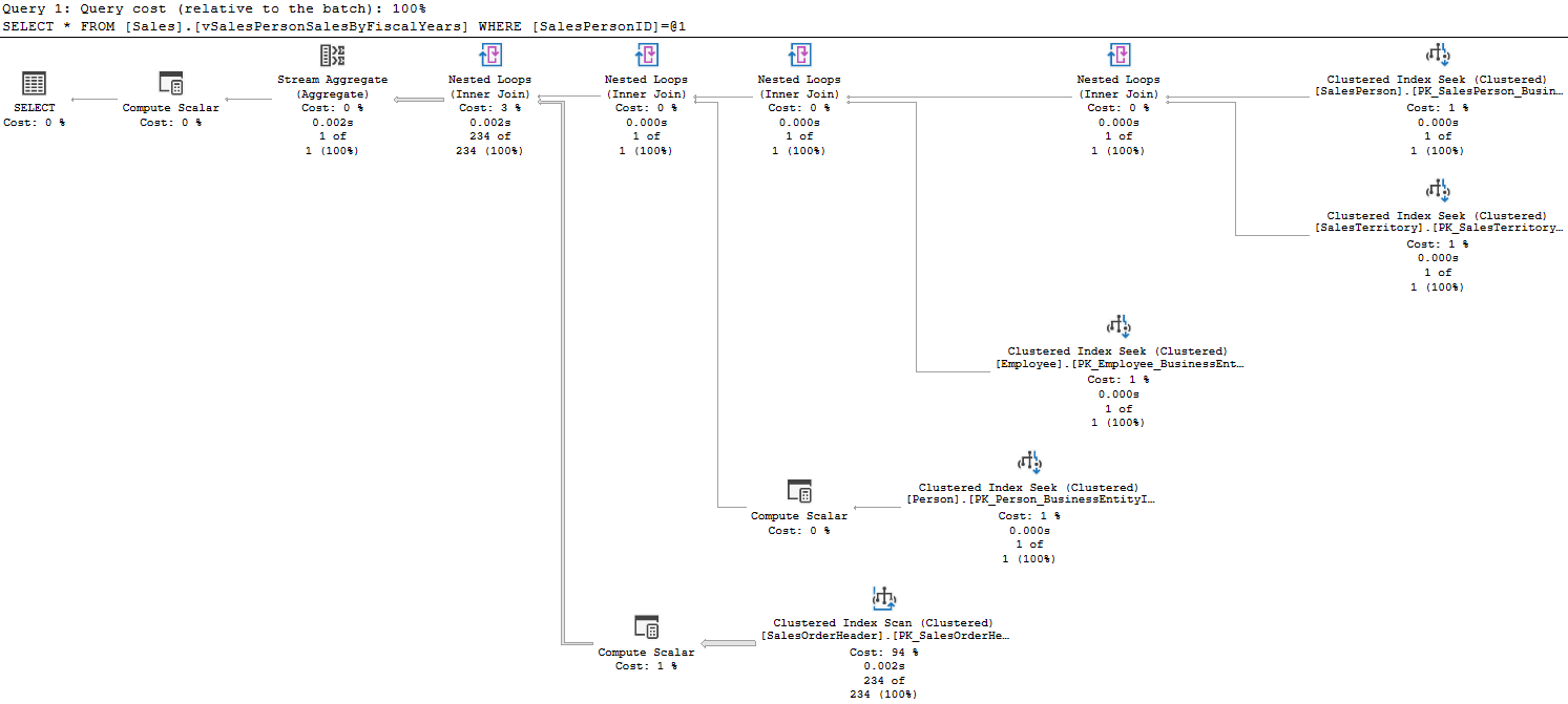
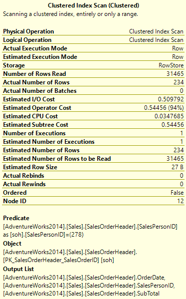
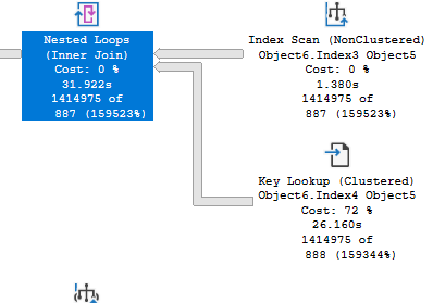
I reviewed a garbage collection process that’s been in place for some time. The procedure populates a temp table with the key values for the table that is central to the GC. We use the temp table to delete from the related tables, then delete from the primary table. However, the query populating our temp table was taking far too long, 84 seconds when I tested it. 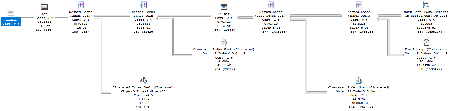 We’re scanning and returning 1.4 million rows from the first table, doing a key lookup on all of them. We scan another table to look up the retention period for the related account, as this database has information from multiple accounts, and return 8.4 million rows there. We join two massive record sets, then have a filter operator that gets us down to a more reasonable size.
In general, when running a complex query you want your most effective filter, that results in the fewest rows, to happen first. We want to get the result set small early, because every operation after becomes less expensive. Here’s part of our anonymized query:
 WHERE
   Object5.Column10 = ?
   AND Object5.Column6 < Variable4 - COALESCE(Object12.Column1,Variable1,?)
So, Object5 is our main table. Column10 is a status column, and we compare that to a scalar value to make sure this record is ready for GC. That’s fine. The second is checking if the record is old enough to GC, and this is where things get interesting. The code here is odd; we’re subtracting a COALESCE of three values from a DATETIME variable, relying on behavior that subtracting an INT from a DATETIME subtracts that number of days from the DATETIME. There’s an implicit conversion, but it is on the variable side of the inequality. And the plan above appears to be our result.
So, Bad Date Math Code?
Seems like a good root cause, and I don’t like this lazy coding pattern, but let’s test it out with tables we can all look at. Would this be any better if we had written this to use the DATEADD function to do the math properly?
USE AdventureWorks2014
GO
--CREATE INDEX IX_SalesOrderHeader_ModifiedDate ON Sales.SalesOrderHeader (ModifiedDate);

SELECT TOP 100
	soh.ModifiedDate,
	soh.SalesOrderID
FROM Sales.SalesOrderHeader soh
WHERE
	soh.ModifiedDate < DATEADD(day, -1, GETUTCDATE());

SELECT TOP 100
	soh.ModifiedDate,
	soh.SalesOrderID
FROM Sales.SalesOrderHeader soh
WHERE
	soh.ModifiedDate < GETUTCDATE() - 1;
So, if we had an index on the OrderDate column, would it perform differently?
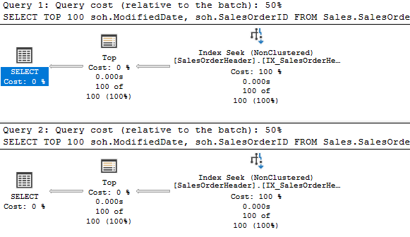
Apparently not. Same plan, same cost. But when you think about it, this tests the date math by subtracting an integer from the DATETIME provided by GETUTCDATE(). The original was subtracting a COALESCE of three values. One of those values was a float. Could the COALESCE or the resulting data type have made this more complicated?
Testing COALESCE
USE AdventureWorks2014
GO
DECLARE
	@AccoutSetting FLOAT = 8.0,
	@Default INT = 365;

SELECT TOP 100
	soh.ModifiedDate,
	soh.SalesOrderID
FROM Sales.SalesOrderHeader soh WITH(INDEX(IX_SalesOrderHeader_ModifiedDate))
WHERE
	soh.ModifiedDate < DATEADD(DAY, -COALESCE(@AccoutSetting, @Default), GETUTCDATE());
Running this, again we see a nice seek that reads and returns 100 rows. So the different data type and the COALESCE makes no difference.
Looking at the original query again, the first value isn’t a variable, it’s a column from a different table. We can’t filter by this column until we’ve read the other table, which affects our join order. But we have no criteria to seek the second table with.
Joined Filtering
One more test. Let’s see what the behavior looks like if we join to the Customers table to look for the RetentionPeriod. First, I’ll create and populate some data in that column:
USE AdventureWorks2014
GO
IF NOT EXISTS(
	SELECT 1
	FROM INFORMATION_SCHEMA.COLUMNS isc
	WHERE
		isc.TABLE_NAME = 'Customer'
		AND isc.TABLE_SCHEMA = 'Sales'
		AND isc.COLUMN_NAME = 'RetentionPeriod'
)
BEGIN
	ALTER TABLE Sales.Customer
		ADD RetentionPeriod INT NULL;
END;
GO
UPDATE TOP (100) sc
	SET sc.RetentionPeriod = (sc.CustomerID%4+1)*90
FROM Sales.Customer sc;
GO
CREATE INDEX IX_Customer_RetentionPeriod ON Sales.Customer (RetentionPeriod);
GO
I only populated a few of the records to better match the production issue; only some accounts have the value I’m looking for, hence the COALESCE.
USE AdventureWorks2014
GO
DECLARE
	@Default INT = 365;

SELECT TOP 100
	soh.ModifiedDate,
	soh.SalesOrderID,
	sc.RetentionPeriod
FROM Sales.SalesOrderHeader soh
LEFT JOIN Sales.Customer sc
	ON sc.CustomerID = soh.CustomerID
	AND sc.RetentionPeriod IS NOT NULL
WHERE
	soh.ModifiedDate < DATEADD(DAY, -COALESCE(sc.RetentionPeriod, @Default), GETUTCDATE());
Now we’re trying to filter records in SalesOrderHeader, based on the Customer’s RetentionPeriod. How does this perform?
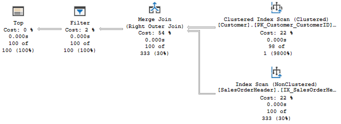
Well, the row counts aren’t terrible, but we are scanning both tables. The optimizer opted to start with Customer table, which is much smaller. We’re not filtering on the date until the filter operator, after the merge join.
I’d be worried that with a larger batch size or tables that don’t line up for a merge join, we’d just end up doing a hash match. That would force us to scan the first table, and without any filter criteria that would be a lot of reads.
Solution
The solution I applied to my production query was to create a temp table that had the account ID and the related retention period. I joined this to my primary table, and the query that was taking 84 seconds was replaced with one that took around 20 milliseconds.
USE AdventureWorks2014
GO
IF OBJECT_ID('tempdb..#AccountDates') IS NULL
BEGIN
	CREATE TABLE #AccountDates(
		CustomerID INT,
		GCDate DATETIME
	);
END
GO
DECLARE
	@Default INT = 365;

INSERT INTO #AccountDates
SELECT
	sc.CustomerID,
	DATEADD(DAY, -COALESCE(sc.RetentionPeriod, @Default), GETUTCDATE()) AS GCDate
FROM Sales.Customer sc
WHERE
	sc.RetentionPeriod IS NOT NULL;

SELECT
	soh.SalesOrderID
FROM #AccountDates ad
JOIN Sales.SalesOrderHeader soh
	ON soh.CustomerID = ad.CustomerID
	AND soh.ModifiedDate < ad.GCDate;

TRUNCATE TABLE #AccountDates;
GO
Here’s how I’d apply that thought to our example. I’ve created a temp table with CustomerID and its associated RetentionDate, so we could use that to search Sales.SalesOrderHeader.
You may have noticed my filter on the Sales.Customer table. In the live issue, the temp table had dozens of rows for dozens of accounts, not the tens of thousands I’d get from using all rows Sales.Customer in my example. So, I filtered it to get a similar size in my temp table.
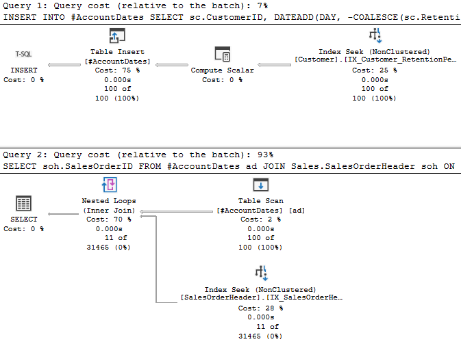
Infinitely better. Literally in this case, since the ElapsedTime and ActualElapsedms indicators in the plan XML are all 0 milliseconds. I’m declaring victory.
If you liked this post, please follow me on twitter or contact me if you have questions.