Optimizer, SQLJared

Understanding Cost in SQL Server

Cost is an important concept in SQL Server. It is key in how plans are compared and chosen by the optimizer, and it can guide us to problem operators as we tune a query’s performance. It can also lead us astray if we follow it blindly. In this post, I want to explain what cost is and how we use it.

Many queries (that aren’t trivial) can be executed in a number of different ways. Each index on a table is a possible path for the optimizer to use, and statistics allow the optimizer to determine the cost of a given operation. SQL Server determines what potential plan it will use in large part based on cost. The optimizer isn’t exhaustive. It won’t compare all possible plans; that would take too long.

Let’s take a look at an example query from the AdventureWorks database.


SELECT * FROM Sales.vSalesPersonSalesByFiscalYears 
WHERE SalesPersonID=278

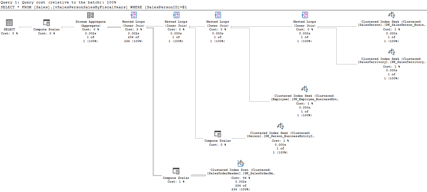
There is a cost provided for each query relative to the batch; that can help you narrow down which statement is the issue if a large batch or procedure is performing poorly. This query is in the only one in the batch.

This query hits 5 tables, and has a number of joins and other operations. Each operation has a cost displayed here as a percentage of the total query. You’ll notice one operation has a cost of 94%; let’s zoom in.

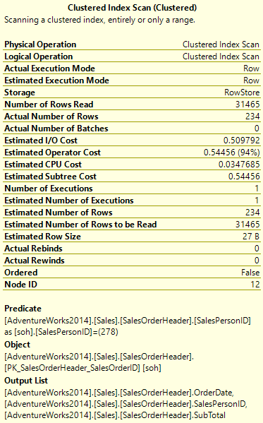
This has a cost of 0.54456. This is broken further into an I/O Cost and a CPU Cost. There is also a Subtree Cost, which would include any operators that feed into this one, but in this case there aren’t any. The operator returned 234 rows, but it read over 31k. So the cost seems appropriate; we really are doing some work here.

The number for cost is always presented without a unit, you may ask 0.54456 of what exactly? Pounds? Parsecs?

Calibration

The story as I recall was that cost was derived from how long it took an early developer of SQL Server to run a given operation on his desktop computer, in seconds. So initially cost was expressed in seconds, but that’s not the case anymore. It’s a more generic expression of how much work is involved in executing the operation.

Given the cost value is fairly generic, you need an idea of what is a cheap operator or an expensive one. Here’s one of the other index seeks from the query above.

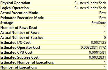
So, we’re doing an index seek not a scan. We not only returned 1 row, we only read one row. In terms of reading a normal table, it’s not going to get any cheaper than this. This cost of about 0.003 is something you’ll see many times for that reason.

So, what constitutes an expensive query? That’s a matter of opinion. You could gauge this by the “Cost Threshold for Parallelism” setting in SQL Server. This is a server level setting that sets how expensive an operation has to be for SQL Server to consider going parallel to perform it. The default setting is 5, so you could argue that’s an expensive query. But this setting is probably quite low for current servers. I think at work, this setting is 100 for most of the servers I work on.

Keep in mind, the cost threshold is for the operation, not the entire plan.

Cost isn’t exact

One thing to remember is that cost in SQL Server is always an estimate. This is a number SQL Server calculates when considering multiple potential plans to determine which would be the best. But the number of rows it expects a given operation to return or how many times that operation runs can be off. All of that is based on statistics.

It doesn’t then go back and update the cost number later if those numbers were incorrect. So while we can use the cost as an indicator of which query or operator we should focus on, don’t completely tunnel-vision that one thing.

I could talk at this point about estimated plans versus actual plans, but fortunately Grant Fritchey has already done so. The gist of his post is that an actual plan is one that has actual runtime metrics. For example, “Number of Rows Read”, “Actual Number of Rows”, and “Number of Executions” in the images above.

It’s helpful to have plans with these actual numbers; they can help you confirm if the costs look accurate. “Number of Rows Read” is the main data point I look at most of the time.

You may also find the following situation in plans as you look at them:

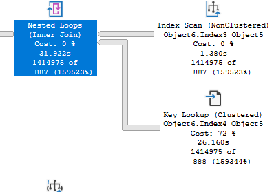
The optimizer estimated 887 or 888 rows for these operators, but the number of rows returned is much higher. So the cost of 72% for the one operator isn’t really accurate. That operator read and returned many more rows, as did the other related operators. If you saw an estimated plan without these runtime numbers, you may come away with a very different impression of how this query is running.

Conclusion

I’ve always felt cost is not well explained, so hopefully this post will help answer some questions. Understanding cost can be really helpful in troubleshooting poorly performing queries, but don’t focus solely on it when analyzing a problem.

If you liked this post, please follow me on twitter or contact me if you have questions.

The transitive Property

You may recall the transitive property from elementary school math class. It states:

If A = B, and B = C, then A = C

The SQL Server optimizer can and will use this property, and it can lead to issues in your queries. When I’m writing a query, I have a clear idea of how I want it to operate. But using the transitive property, SQL Server has additional options one might not expect, and this may occasionally cause things to go awry. Consider this:


DECLARE @OrderID INT = 110001;

SELECT 
	so.CustomerID,
	so.OrderID,
	so.CustomerPurchaseOrderNumber,
	sol.OrderLineID,
	sol.StockItemID,
	sol.Quantity,
	sol.UnitPrice
FROM Sales.Orders so
JOIN Sales.OrderLines sol
	ON sol.OrderID = so.OrderID
WHERE
	so.OrderID = @OrderID;

I’d expect the optimizer to seek the Orders table, then join to OrderLines. But since @OrderID is also equal to sol.OrderID, it could start the query there. There would be little difference; the OrderID column is indexed in both tables and neither table is that large. There’s only 3 OrderLines for this OrderID.

But what if:

The CustomerID was present in all tables. And was part of the primary key in each.

The data set was larger, with 100’s of millions of rows in our OrderLines table.

Statistics were last updated by an auto-update. A table of this size would have a very small sampling rate by default, <1%.

Our database has a large number of customers, and we’re running a query to get recent orders for a large customer that haven’t been picked yet.

We may end up with a query like this:


DECLARE 
	@CustomerID INT = 55;

SELECT 
	so.CustomerID,
	so.OrderID,
	so.CustomerPurchaseOrderNumber,
	so.OrderDate,
	sol.OrderLineID,
	sol.StockItemID,
	sol.Quantity,
	sol.UnitPrice
FROM Sales.Orders so
JOIN Sales.OrderLines sol
	ON sol.OrderID = so.OrderID
	AND sol.CustomerID = so.CustomerID
WHERE
	so.CustomerID = @CustomerID
	AND so.OrderDate > DATEADD(DAY,-90,GETDATE())
	AND so.PickingCompletedWhen IS NULL;

If our PK has the CustomerID first, we could use that to search either table. If we don’t have an index with the CustomerID and our dates on Orders, those fields will be in our predicate, not our seek predicate. With poor statistics, the optimizer may seek OrderLines first, returning all lines for that customer, before later joining an filtering it down. In this situation, that could be a mountain of reads.

Countering The transitive Property

So what if you experience or anticipate this issue with a query? I see a few approaches to prevent the bad plan from sneaking up on your server.

Join Hints or Force Order: The FORCE ORDER hint would direct the optimizer to hit the Orders table first. A join hint like INNER LOOP JOIN would set the join type, and also force the order. Either would results in seeking the Orders table before joining to OrderLines, preventing our worst case.

Index hints: If you hint the optimizer to use an index based on CustomerID and OrderDate, that would point it in the direction of using the Orders table first, avoiding the problem.

Better stats: An argument can definitely be made to not use auto-updated stats on a sufficiently large table. I’ve seen sampling rates below 0.1%, and mistakes can be made then. If you updated stats with a large sampling rate, the optimizer will have better information to work with, and that may avoid the worst case.

I thought this property of the optimizer was interesting when I first saw it in play, and I haven’t seen it referred to much. Hopefully this post will give you a little more insight into what the optimizer can do, and how we sometimes need to respond.