Update and Correction:

This blog was originally posted on February 20. Since then I read other articles that suggested different behavior with the Halloween Problem. I contacted Paul White, who informed me that the WideWorldImporters database uses compatibility level 130 (SQL Server 2016) by default. So, I tested on a SQL Server 2019 instance but was probably seeing an issue addressed in later updates.

I tested again at compatibility level 150 and saw a different execution plan which led to different conclusions.

I’ve left the majority of the post unchanged, but I’m adding an addendum section, and updating the summary and its conclusions. So, make sure you read those sections for the corrections.

Original Post:

I find myself talking about the Halloween Problem a lot and wanted to fill in some more details on the subject. In short, the Halloween Problem is a case where an INSERT\UPDATE\DELETE\MERGE operates on a row more than once, or tries to and fails. In the first recorded case, an UPDATE changed multiple rows in the table more than once.

So let’s take a look at an example using a publicly available database, WideWorldImporters.

A Halloween Problem example

Here’s a simple update procedure. We’re going to update the quantity for an item in the Sales.OrderLines table:

CREATE OR ALTER PROCEDURE Sales.OrderLines_UpdateQuantity
	@OrderID INT,
	@StockItemID INT,
	@Quantity INT
	WITH EXECUTE AS OWNER
AS
BEGIN
	SET NOCOUNT ON;
	SET XACT_ABORT ON;

	UPDATE sol
	SET
		sol.Quantity = @Quantity,
		sol.PickedQuantity = @Quantity
	FROM Sales.OrderLines sol
	WHERE
		sol.OrderID = @OrderID
		AND sol.StockItemID = @StockItemID;
		-- AND sol.Quantity <> @Quantity;
END;
GO

You may notice the commented line. In one description of the Halloween Problem I heard\read, it was suggested that if we try to SET something that is in our WHERE clause the problem is likely to occur. Or rather, SQL Server will see the possibility of the problem and add protections to our execution plan to prevent it.

First, let’s test without that line, and see what our execution plan tells us.

EXEC Sales.OrderLines_UpdateQuantity
	@OrderID = 5,
	@StockItemID = 155,
	@Quantity = 21;
GO

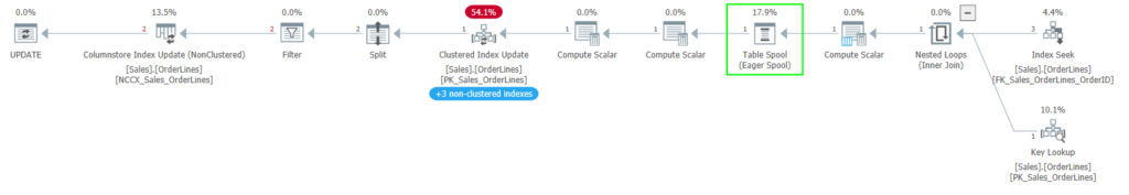
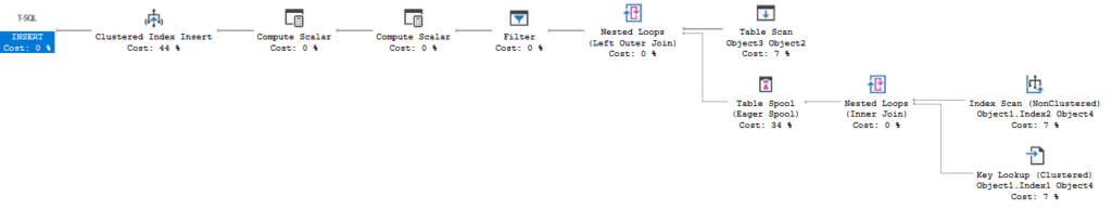
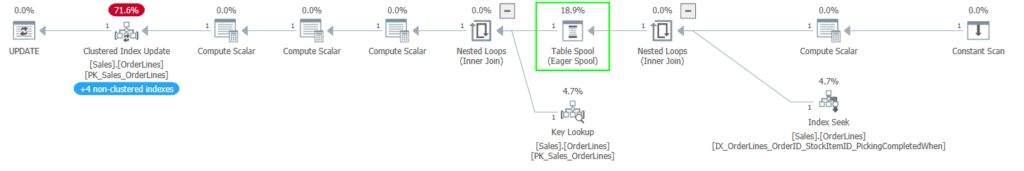
The eager spool between our index reads and clustered index update shows that SQL Server added Halloween protections to prevent the problem. The problem is prevented by separating the read phase of the query from the write phase.

This usually involves a blocking operator. Most often this is an eager spool, but if there is another blocking operator in the plan like a sort or hash match, that blocking operator may remove the need for a separate spool.

The Halloween Problem would occur if a query is running in row mode and as rows are still being read, rows are being updated and moved in an index. This allows the read operation to potentially read the updated row again and operate on it again. The index movement is key in this scenario.

But with a blocking operator between the read operation and the write, we force all the reads to complete first. This gives us a complete, distinct list of rows to be updated (in this example) before we get to the clustered index update, so it isn’t possible to update the same row twice.

So, how does index movement come into play here? We are updating the Quantity and PickedQuantity columns in our UPDATE statement. Both fields are key columns in the only columnstore index on the table, NCCX_Sales_OrderLines.

CREATE NONCLUSTERED COLUMNSTORE INDEX [NCCX_Sales_OrderLines] ON [Sales].[OrderLines]
(
[OrderID],
[StockItemID],
[Description],
[Quantity],
[UnitPrice],
[PickedQuantity]
)WITH (DROP_EXISTING = OFF, COMPRESSION_DELAY = 0) ON [USERDATA];
GO

So when we update these columns, the affected rows will move in that index. If the row moves, that means a read operation could continue reading and find the same row again, returning it as a part of its result set a second time.

Interestingly, we aren’t reading from the columnstore index in the plan provided. Since that’s the only index containing these columns as key values, it’s the only index where the rows should move. In this case, our read operators shouldn’t encounter updated rows a second time, since they use the FK_Sales_OrderLines_OrderID (with a key lookup against PK_Sales_OrderLines).

I wonder if SQL Server decided the Halloween protections were needed before it decided which index it would use for the read.

Removing the index

Either way, if we dropped the NCCX_Sales_OrderLines index, we should see a plan without an eager spool between the read operators and the update operator.

IF EXISTS(
	SELECT 1
	FROM sys.indexes si
	WHERE
		si.name = 'NCCX_Sales_OrderLines'
)
BEGIN
	DROP INDEX [NCCX_Sales_OrderLines]
		ON Sales.OrderLines;
END;
GO

With the index removed, let’s look at the new plan.

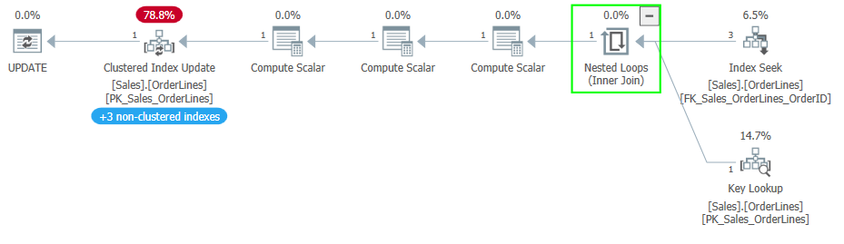
We’ve lost the extra steps to the left of the clustered index update operator to update the columnstore index, and we have also lost the eager spool between the read operators and the update operator. This shows without the index movement, Halloween protections are no longer needed.

Performance impact of protections

Let’s look at the data from Query Store to see how big the difference is between the two execution plans.

I ran a simple query against the same OrderID in Sales.OrderLines before running the procedure before and after the index change to get the data into the cache (because cold cache issues were making a large difference). I also ran the procedure 10 times to try to average out our results in case any odd wait types were seen.

80 microseconds versus 46 microseconds. Blazing fast in both cases with the data already cached, but the plan with Halloween protections took 74% longer. Unsure if the update to a columnstore index is significantly more expensive than that of a rowstore index. Perhaps we should test this again without columnstore complicating the issue.

Speaking in general, I would expect a bigger difference in a query affecting more rows. For a query that only returns 3 rows from the first index seek, the delay caused by the spool would be very small. But imagine if we have a query that reads tens or hundreds of thousands of rows before performing its write operation.

Normally such a query would be passing rows it has read up to the join and update operators while it is continuing to read. Those operations would be happening on different threads in parallel.¹

If we are being protected from the Halloween Problem, the eager spool will not return any rows to the operations above it (like the clustered index update) until all rows have been read. So the writes cannot start until much later, and the more rows being read the more considerable the delay.

Nonclustered indexes?

If you noticed the “+3 non-clustered indexes” banner in one of the plans above, that’s indicating the nonclustered indexes updated when we updated the clustered index. This is more obvious in Plan Explorer than in the plans as shown in SQL Server Management Studio. So, I wanted to point that out in case the visual was confusing to anyone.

But this raises another question. If we are updating those indexes, why don’t they cause the Halloween protections to be used?

That is because the quantity columns are present in those indexes only as included columns. Changes to those columns won’t affect where the row sorts, but the values still need to be updated.

Rowstore testing

So, let’s see how this looks with a rowstore index. Here’s a second procedure, similar to the first but also updating PickingCompletedWhen.

CREATE OR ALTER PROCEDURE Sales.OrderLines_UpdateQuantityWhen
	@OrderID INT,
	@StockItemID INT,
	@Quantity INT
	WITH EXECUTE AS OWNER
AS
BEGIN
	SET NOCOUNT ON;
	SET XACT_ABORT ON;

	UPDATE sol
	SET
		sol.Quantity = @Quantity,
		sol.PickedQuantity = @Quantity,
		sol.PickingCompletedWhen = GETUTCDATE()
	FROM Sales.OrderLines sol
	WHERE
		sol.OrderID = @OrderID
		AND sol.StockItemID = @StockItemID
		AND sol.PickingCompletedWhen < GETUTCDATE();
END;
GO

Initially, no index uses PickingCompletedWhen. So if we execute the procedure as is, we shouldn’t see the tell-tale eager spool.

EXEC Sales.OrderLines_UpdateQuantityWhen
	@OrderID = 5,
	@StockItemID = 155,
	@Quantity = 21;
GO

This plans is what we’d expect. If we add an index, how does this change the plan and how does this change the performance?

IF NOT EXISTS(
	SELECT 1
	FROM sys.indexes si
	WHERE
		si.name = 'IX_OrderLines_OrderID_StockItemID_PickingCompletedWhen'
)
BEGIN
	CREATE INDEX IX_OrderLines_OrderID_StockItemID_PickingCompletedWhen
		ON Sales.OrderLines (OrderID, StockItemID, PickingCompletedWhen);
END;
GO

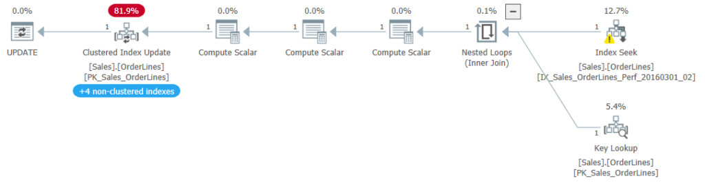
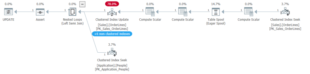
Here, we see the eager spool implementing the Halloween protections again, but between the index seek and the key lookup. Note that the new index is the one we are using for the index seek. The clustered index update now indicates it is updating 4 nonclustered indexes, including the new index.

So, is the performance difference as stark as it was with the columnstore index?

So, 52 µs vs 118 µs. The query took about ~126% longer when the Halloween protections were present. More than we saw with the columnstore index, which is surprising. Perhaps it is relevant that we are updating a third field. It almost feels like the observer effect at this scale.

Addendum

So, to correct things here, let’s go back to the first procedure.

CREATE OR ALTER PROCEDURE Sales.OrderLines_UpdateQuantity
	@OrderID INT,
	@StockItemID INT,
	@Quantity INT
	WITH EXECUTE AS OWNER
AS
BEGIN
	SET NOCOUNT ON;
	SET XACT_ABORT ON;

	UPDATE sol
	SET
		sol.Quantity = @Quantity,
		sol.PickedQuantity = @Quantity
	FROM Sales.OrderLines sol
	WHERE
		sol.OrderID = @OrderID
		AND sol.StockItemID = @StockItemID;
		-- AND sol.Quantity <> @Quantity;
END;
GO

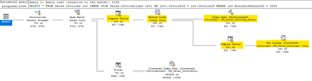
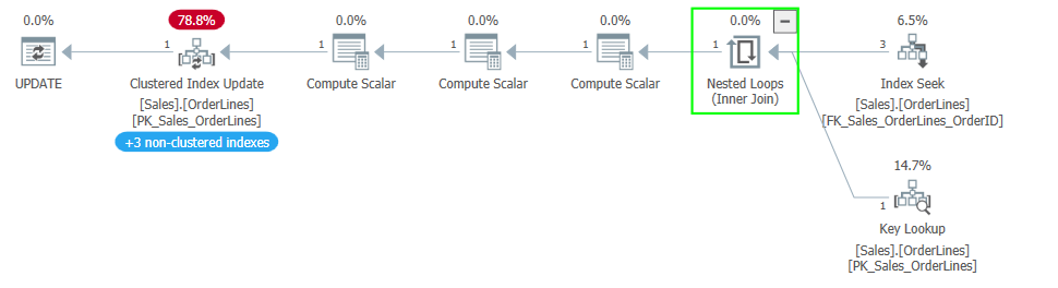
If I run this procedure again with the restored database and no other changes besides updating the compatibility level to 150, I see the following execution plan:

So, we have no eager spool, which means the Halloween Problem isn’t a problem now.

Previously, there was a spool between the index seek and lookup and the clustered index update. The only index using any of the updated fields as a key value was the columnstore index. This suggested that the optimizer will use Halloween protections if any index uses the updated fields as a key value because the rows would be moved in that index.

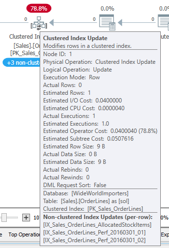
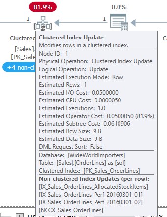
This new plan disproves that because the optimizer no longer uses the protections with the later compatibility level. And the columnstore index (NCCX_Sales_OrderLines) is still present (as you can see if you hover over the clustered index update operator).

As for the second procedure, I see the Halloween protections even without the index I added in my example. Without that index, the query originally used the FK_Sales_OrderLines_OrderID index to seek the rows in question. At the higher compatibility level, the IX_Sales_OrderLines_Perf_20160301_02 index is used, which is keyed on (StockItemID, PickingCompletedWhen).

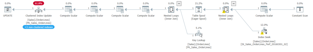
So, the Halloween protections are used because we read from an index keyed on one of the updated fields, and rows being updated will potentially move in that index.

We’ve seen the Halloween protections when using nonclustered indexes so far, but what if we are using the clustered index for the read?

I wrote a quick procedure to change the OrderLineID, which is the only column in the clustered primary key for this table. And this matches expectations; we see the eager spool between the clustered index seek and the update operator.

Summary

Hopefully, the addendum corrects the matter while keeping things clear. I’m updating one of the bullet points below, as well.

It seems there are only two criteria for the protections against the Halloween Problem to be used for an UPDATE query:

1. The object being updated must also be in the query.
2. A column being updated must be a key column in at least one index on the table. One of the updated columns must be a key value in the index used for the read portion of the query, so that the rows may move in that index.

For other statements, the setup is more complex. I find the UPDATE statement is the most straightforward example of the Halloween Problem. But you can see the protections in place if you query from a table as part of an INSERT or DELETE (or MERGE) where you change that same table.

And if we see Halloween protections in the plan for a query, we could change the offending index or the query to change the behavior.

Or we could use the manual Halloween technique, which I will discuss next time.

Thanks again to Paul White for pointing out the compatibility level; I doubt that would ever have occurred to me.

Please contact me if you have any questions or comments. I’ve updated my social media links above to include Counter.Social and Mastodon. We’ll see if there is more #sqlfamily activity on those platforms going forward.

Footnotes

1: Not the type of parallelism we typically think of with SQL Server. Parallelism is typically when a given operation, like an index scan, is expected to process many rows, and SQL Server dedicates multiple threads to that operator or group of operators. In this case, I say parallel because different operators (the index seek, nested loops join, and clustered index update) are all processing rows at the same time, one row at a time.

Another Example: 

I was reviewing the performance of a procedure recently and stumbled over another pumpkin. 

My last blog post was about the Halloween Problem, and we saw its effects on an UPDATE statement. In this case, it was the same issue but with an INSERT statement. Here’s the code being executed:

INSERT INTO Schema1.Object1 (
		Column1,
		Column2,
		Column3,
		Column4 )
	SELECT
		Object2.Column1,
		Object2.Column2,
		Object2.Column3,
		Object2.Column4 
	FROM Object3 Object2
	LEFT LOOP JOIN Schema1.Object1 Object4 WITH(INDEX(Column5))
		ON Object4.Column3 = Object2.Column3
		AND Object4.Column1 = Object2.Column1
		AND Object4.Column2 = Object2.Column2
		AND Object4.Column4 = Object2.Column4
	WHERE
		Object4.Column6 IS NULL

The gist is, we’re trying to insert a record into Object1, assuming said record doesn’t already exist. We’re querying the data we want to insert from a temp table, but joining to the base table to make sure a record doesn’t already exist with the same values.

In the case of an UPDATE statement, if we update fields that are in our query’s search criteria, we could update the same row multiple times. SQL Server’s Halloween protections prevent this, but result in extra work that affect our performance.

The INSERT statement here is similar, trying to insert a record while querying to see if the same record exists. So, again SQL Server adds Halloween protections to our plan:

Plan Analysis

I would have expected us to scan the temp table, then have a LEFT JOIN to the base table. The Table Spool is the red flag that we have an issue with the plan, and is frequently seen with Halloween protections.

The index scan on the base table seems to be overkill since we’re joining on the primary key columns (the key lookup isn’t much of a concern). But we’re likely doing the scan because of the spool; it’s SQL Server’s way of getting all relevant records in one place at one time, breaking the normal flow of row mode operation, to make sure we don’t look up the same record multiple times.

Easy Fix

The data we are trying to insert is being passed into the procedure using a memory-optimized table valued parameter. We’ve queried that into the temp table as another step before our final INSERT SELECT query, because SQL Server will sometimes make poor optimizations when TVP’s are involved (because they have no statistics).

The solution then is an easy one. We move our LEFT JOIN out of the final INSERT, and we make that check as we query the TVP’s data into the temp table. We separate the SELECT against that table from the INSERT; they are now in separate operations, and the Halloween protections are no longer necessary.

If you liked this post, please follow me on twitter or contact me if you have questions.