Hash Match Joins

When I began working at Microsoft, I was very much a novice at performance troubleshooting. There was a lot to learn, and hash match joins were pointed out to me multiple times as the potential cause for a given issue. So, for a while I had it in my head, “hash match == bad”. But this really isn’t the case.

Hash matches aren’t inefficient; they are the best way to join large result sets together. The caveat is that you have a large result set, and that itself may not be optimal. Should it be returning this many rows? Have you included all the filters you can? Are you returning columns you don’t need?

If SQL Server is using a hash match operator, it could be a sign that the optimizer is estimating a large result set incorrectly. If the estimates are far off from the actual number of rows, you likely need to update statistics.

Let’s look at how the join operates so we can understand how this differs from nested loops

How Hash Match Joins Operate

Build Input

A hash match join between two tables or result sets starts by creating a hash table. The first input is the build input. As the process reads from the build input, it calculates a hash value for each row in the input and stores them in the correct bucket in the hash table.

Creating the hash table is resource intensive. This is efficient in the long run, but is too much overhead when a small number of rows are involved. In that case, we’re better off with another join, likely nested loops.

If the hash table created is larger than the memory allocation allows, it will “spill” the rest of the table into tempdb. This allows the operation to continue, but isn’t great for performance. We’d rather be reading this out of memory than from tempdb.

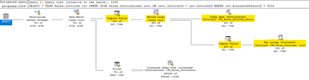
The building of the hash table is a blocking operator. This means the normal row mode operation we expect isn’t happening here. We won’t read anything from the second input until we have read all matching rows from the build input and created the hash table. In the query above, our build input is the result of all the operators highlighted in yellow.

Probe Input

Once that is complete, we move on to the second input in the probe phase. Here’s the query I used for the plan above:

USE WideWorldImporters
GO

SELECT *
FROM Sales.Invoices inv
INNER JOIN Sales.InvoiceLines invl
	ON invl.InvoiceID = inv.InvoiceID
WHERE
	inv.AccountsPersonID = 3002
GO

The build input performed an index seek and key lookup against Sales.Invoices. That’s what the hash table is built on. You can see from the image above that this plan performs a scan against Sales.InvoiceLines. Not great, but let’s look at the details.

There is no predicate or seek predicate, and we are doing a scan. This seems odd if you understand nested loops, because we are joining based on InvoiceID, and there is an index on InvoiceID for this table. But the hash match join operated differently, and doesn’t iterate the rows based on the provided join criteria. The seek\scan against the second table has to happen independently, then we probe the hash table with the data it returns.

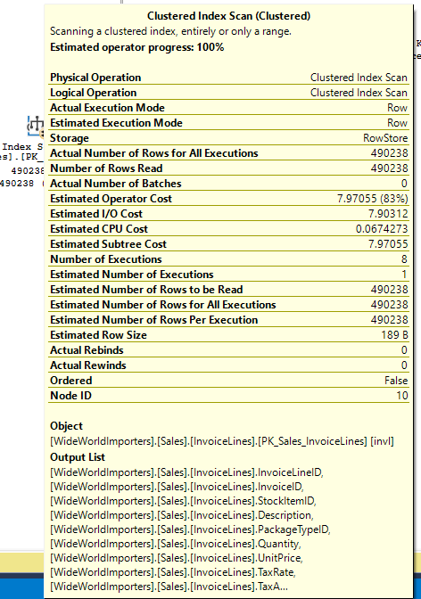
If the read against Sales.InvoiceLines table can’t seek based on the join criteria, then we have no filter. We scan the table, reading 490,238 rows. Also unlike a nested loop join, we perform that operation once.

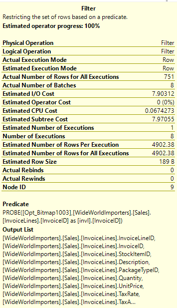
There is a filter operator before the hash match operator. For each row we read of Sales.InvoiceLines, we create a hash value, and check against the hash table for a match. The filter operator reduces our results from 490,238 rows to 751, but doesn’t change the fact that we had to read 490,238 rows to start with.

In the case of this query, I’d want to see if there’s a filter I can apply to the second table. Even if it doesn’t change our join type away from a hash match, if we performed a seek to get the data initially from the second table, it would make a huge difference.

Remember Blocking Operators?

I mentioned the build input turns that branch of our execution plan into a blocking operator. This is something try to call out the normal flow of row mode execution.

With a nested loops join, we would be getting an individual row from the first source, and doing the matching lookup on the second source, and joining those rows before the join operator asked the first source for another row.

Here, our hash match join has to gather all rows from the first source (which here includes the index seek, key lookup, and nested loops join) before we build our hash table. This could significantly affect a query with a TOP clause.

The TOP clause stops the query requesting new rows from the operators underneath it once it has met it’s requirement. This should result in reading less data, but a blocking operator forces us to read all applicable rows first, before we return anything to upstream operators.

So if your TOP query is trying to read a small number of rows but the plan has a hash match in it, you will be likely reading more data that you would with nested loops.

Summary

Actual numbers comparing join types would depend a ton on the examples. Nested loops are better for smaller result sets, but if you are expecting several thousand (maybe ten or more) rows read from a table, hash match may be more efficient. Hash matches are more efficient in CPU usage and logical reads as the data size increases.

I’ll be speaking at some user groups and other events over the next few months, but more posts are coming.

As always, I’m open to suggestions on topics for a blog, given that I blog mainly on performance topics. You can follow me on twitter (@sqljared) and contact me if you have questions. You can also subscribe on the right side of this page to get notified when I post.

Have a good night.