In my previous blog, I set up a database with two tables, one with a large CHAR(8000) field and one with a smaller VARCHAR(100) field. Both tables use an INT IDENTITY column for their primary key. Since we’ll be inserting rows sequentially, we will see page latch contention when multiple threads attempt to insert.

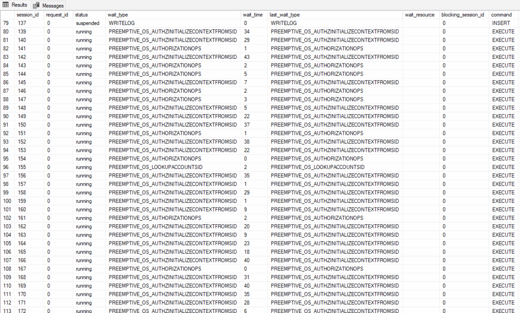
We ran some initial tests with SQLQueryStress to create some page latch contention and resolved an odd problem causing connection delays.

We’ll use these two tables and test several different approaches to reduce page latch contention.

OPTIMIZE_FOR_SEQUENTIAL_KEY

This is an option you can use when building an index. This option attempts to control the number of new requests and keep the throughput high. SQL Server does this by prioritizing queries that can complete more quickly.

You will see a drop in PAGELATCH waits, but that’s because they are partly replaced with BTREE_INSERT_FLOW_CONTROL waits. We should include those in our results.

To test this, I’ll need to drop the PK on my existing tables and rebuild them with this option (you could rebuild a clustered index that isn’t a constraint).

For each test, I’ll insert 100 times across each of 100 threads to create a total of 10,000 inserted rows.

Change the clustered index

Since our clustered index is sequential, one option is to use another column (or group of columns) as the clustered index.

Another highly selective column would be ideal. I used the Price column for this test.

When I first tested this, I had left OFSK enabled for the clustered primary key. When I realized this and dropped\recreated without this option, there was virtually no difference (217µs per execution vs 218µs). A further indication that it doesn’t help here.

But what if we still need the IDENTITY column to be indexed for our queries? We can index that column as a nonclustered index. I’ve seen references to page latch contention in the past that discuss this as a problem for clustered indexes only, but I have seen page latch contention on nonclustered indexes before.

I tested again with the Price clustered index, but with a nonclustered index on the IDENTITY column.

Use a computed column

This is another way of indexing a non-sequential column. What if you don’t have another column you want to base your clustered index on? We can make one up.

--Add the new computed column, ModValue
IF NOT EXISTS(
	SELECT 1 FROM sys.columns sc
	WHERE
		sc.name = 'ModValue'
		AND sc.object_id = OBJECT_ID('Testing.InsertContention_100')	)
BEGIN
	ALTER TABLE Testing.InsertContention_100
		ADD ModValue AS CONVERT(TINYINT, ABS(InsertID%16)) PERSISTED NOT NULL;
END;

The script above adds a computed persisted column. This is based on the InsertID, but run through a modulus operator. This doesn’t prevent insert contention, but it should spread our inserts across 16 pages in the table.

Partition the table

This extends the computed column from the previous example. If we partition based on the ModValue column, we’ll have 16 separate B-tree structures in our clustered index.

Does this give us an advantage over a clustered index on the same column?

Batch your operations

Instead of having a ton of threads each inserting one row, why not insert them all in one call? If your procedure accepts a table variable (I’d suggest a memory-optimized one) as input, the application can provide 100 rows (or more) in a call.

Fewer threads, less contention.

Each INSERT will take longer, but it tends to be far more efficient to write/read 100 rows in a call rather than to write/read 1 row in each of 100 operations.

If each call inserts 100 rows, I want to still insert 10,000 rows as in my other tests. At first, I ran the test with these options.

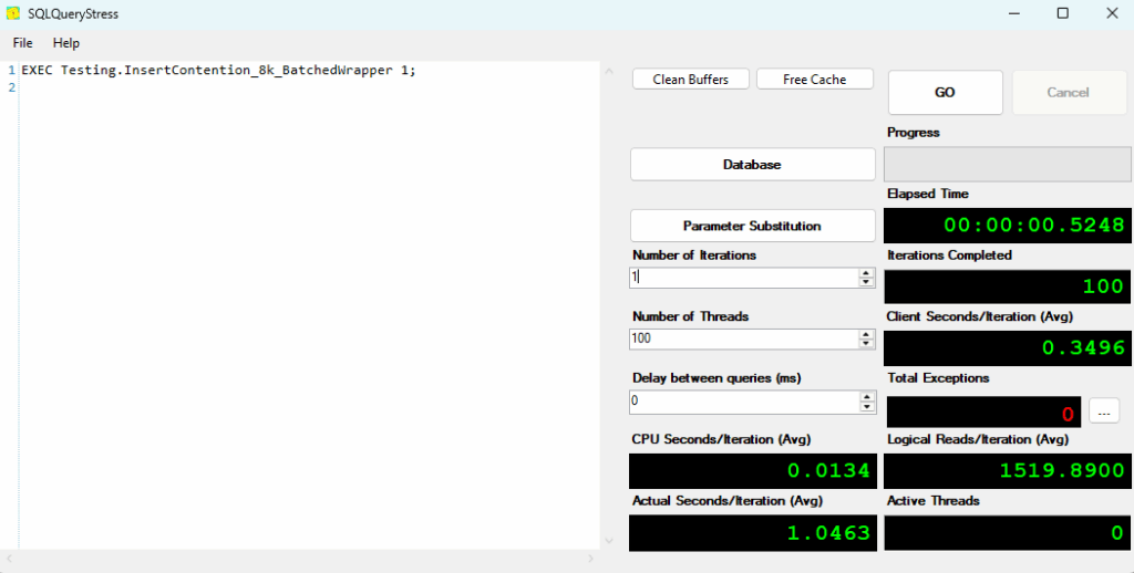
But then I realized my mistake. I had 100 threads call this procedure once, but that’s not the point of batching. I shouldn’t have 100 parallel operations. That may happen if the application receives a large set of data at once and needs to break it down into 100-row chunks.

Otherwise, I would like the application to call as soon as it has 100 rows to insert. So, I ran a second test with 1 thread, but it executed 100 times. This shouldn’t have any page latch contention.

The truth may be in the middle, depending on the inserting application.

Memory-Optimized Table

If the table itself is memory-optimized, we gain optimistic concurrency and remove page latch contention.

Once I saw the result, I decided to do one more variation. I used a memory-optimized table, and batched the inserts into it.

Results

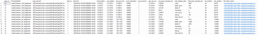
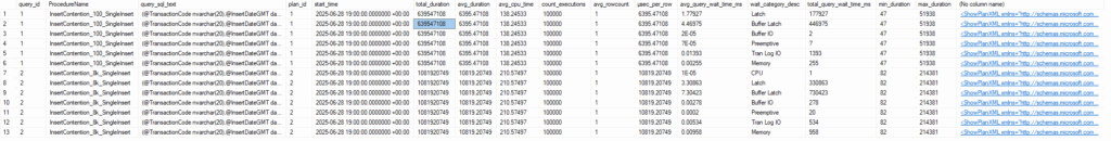
I’ve included my test numbers above. I used separate stored procedures for each test option to make it easy to query the data from Query Store.

• Baseline
  • 33.5 seconds total to insert 10,000 rows into the smaller table, 15.8 seconds of that time is PAGELATCH waits.
  • 53.1 seconds to insert into the larger table, with 35.5 seconds of PAGELATCH waits.
  • CPU time for both is less than 1 second.
• OPTIMIZE_FOR_SEQUENTIAL_KEY
  • Little difference for this option. We spend more time waiting if you include the BTREE_INSERT_FLOW_CONTROL waits (recorded in Query Store as ‘UNKNOWN’), but the duration is slightly lower overall.
  • If all of the inserts are the same, this option can’t really be effective. If there were more of a mix of simple write statements and more complex statements, there would be more to optimize here. When all the INSERT statements are the same, there’s no advantage.
• Non-sequential Clustered
  • Huge improvement.
  • 97.7% duration reduction on the small table.
  • 96.2% duration reduction on the large table.
• Non-sequential Clustered (ID NC)
  • Added a nonclustered index on the InsertID column.
  • Slightly better than the baseline for the small table, and a 24.5% reduction for the large table.
  • The difference between this test and the previous shows that even one sequential index makes a huge difference, even if it is a nonclustered index.
• Mod PK
  • 98.0% duration reduction compared to the baseline for the smaller table.
  • 93.6% duration reduction compared to the baseline for the larger table.
• Partitioned Mod PK
  • Very similar to the previous test in terms of duration.
  • The PAGELATCH waits are lower for the partitioned table compared to simply the mod PK.
• Batched
  • This test has 100 threads. Each thread makes 1 call to insert 100 records. Since this is multi-threaded, there is still page latch contention.
  • Reduced the duration for the smaller table by about 4/5. Only a 1/3 reduction for the large table.
  • The results are better than the baseline, OFSK, and the sequential nonclustered index, but worse than the test with no sequential index or the mod or partitioned PK.
• Batched Single-Threaded
  • This test has 1 thread. It calls a procedure 100 times to insert 100 records per call. Single-threaded, so the 0 for page latch waits is expected.
  • Best result by far to this point. 20x faster compared to the partitioned mod PK.
• Memory-Optimized
  • Inserts into permanent memory-optimized tables. Optimistic concurrency, no PAGELATCH waits.
  • Very good, but several times slower than the batched single-threaded test.
  • Very little difference between the small and large tables. This could be due to differences in how pages are allocated for a memory-optimized table compared with a physical table.
  • Why was the batched approach better? My first thought is the efficiency of having one statement write or read multiple rows.
• Memory-Optimized (Batched)
  • What if we used a memory-optimized table, and our application inserted batches of 100 rows?
  • Slightly faster than the batched single-threaded insert for the smaller table; several times faster for the large table.
  • 22ms to insert 10,000 rows.

Conclusion

Your mileage may vary depending on your server’s configuration, but the results give us three clear tiers.

1. The baseline test, OFSK, and the nonclustered sequential index were all relatively bad. The parallel batched test was nearly as slow for the larger table.
2. Removing all sequential indexes makes a huge difference. Using the mod PK or a partitioned PK based on the mod column is comparable.
3. Memory-optimized tables and batched operations (as long as they aren’t still using a lot of parallel threads) are far more effective.

PAGELATCH waits are a very difficult wait type to address, but hopefully, this will help you fight back against them.

My social media links are above. Please contact me if you have questions, and I’m happy to consult with you if you have a more complex performance issue. Also, let me know if you have any suggestions for a topic for a new blog post.

I’ve already posted a blog on page latch waits and some of the ways to minimize them, but I wanted to add some more on the issue. I wanted to test out some strategies to see how effective they are.

Setting up tests can be very difficult in some cases, and this attempt encountered a very unusual problem. At the risk of delaying the intended results, I wanted to point this out. It’s both interesting and frustrating to work with SQL Server for 20 years and run into new problems.

Setup

I want to recreate the hot page issue, so I need a table to insert into. Do I want to insert large or small rows for this test?

My first thought was to create a table with a char(8000) field, so that each row would fill a page. But surely there would be more contention with a smaller row? If many more rows fit on a page, would more threads insert into the same page, thus giving more contention?

I’m not sure which would be worse, so let’s test both.

USE PageLatch
GO
IF NOT EXISTS(
	SELECT 1 
	FROM sys.schemas ssch
	WHERE 
		ssch.name = 'Testing'
)
BEGIN
	EXEC('CREATE SCHEMA Testing');
END;
GO

IF NOT EXISTS(
	SELECT 1 FROM sys.tables st
	WHERE
		st.name = 'InsertContention_8k'
)
BEGIN
	CREATE TABLE Testing.InsertContention_8k
	(
		InsertID bigint IDENTITY(1,1) PRIMARY KEY,
		TransactionCode CHAR(8000) NOT NULL,
		InsertDateGMT DATETIME NOT NULL,
		Price money NOT NULL,
		Quantity int NOT NULL
	);
END;
GO

IF NOT EXISTS(
	SELECT 1 FROM sys.tables st
	WHERE
		st.name = 'InsertContention_100'
)
BEGIN
	CREATE TABLE Testing.InsertContention_100
	(
		InsertID bigint IDENTITY(1,1) PRIMARY KEY,
		TransactionCode VARCHAR(100) NOT NULL,
		InsertDateGMT DATETIME NOT NULL,
		Price money NOT NULL,
		Quantity int NOT NULL
	);
END;
GO

And we need a simple procedure to insert into each.

CREATE OR ALTER PROCEDURE Testing.InsertContention_8k_SingleInsert
	@TransactionCode nvarchar(20),
	@InsertDateGMT datetime2(2),
	@Price money,
	@Quantity int
	WITH EXECUTE AS OWNER
AS
BEGIN
	SET NOCOUNT ON;
	SET XACT_ABORT ON;

	INSERT Testing.InsertContention_8k
		(TransactionCode, InsertDateGMT, Price, Quantity)
	VALUES
		(@TransactionCode, @InsertDateGMT, @Price, @Quantity);
	RETURN 0;
END;
GO

CREATE OR ALTER PROCEDURE Testing.InsertContention_100_SingleInsert
	@TransactionCode nvarchar(20),
	@InsertDateGMT datetime2(2),
	@Price money,
	@Quantity int
	WITH EXECUTE AS OWNER
AS
BEGIN
	SET NOCOUNT ON;
	SET XACT_ABORT ON;

	INSERT Testing.InsertContention_100
		(TransactionCode, InsertDateGMT, Price, Quantity)
	VALUES
		(@TransactionCode, @InsertDateGMT, @Price, @Quantity);
END;
GO

Originally, I wrote a wrapper procedure to generate random data when called, then call these insert procedures with the payload. I wanted to keep the INSERT as simple as possible, so I didn’t want the data generation to be part of that statement.

After testing with this, I didn’t see as much PAGELATCH contention as I expected. This made me wonder if generating fake data with RAND() and NEWID() calls was too much of the process. The more time I spend generating data, the fewer threads are trying to insert at any given time.

Instead, I wrote a call to insert hard-coded data. Every row is the same, but that should allow us to insert faster.

Unexpected Results

I set up to insert 1000 iterations across 100 threads using SQLQueryStress.

I noticed two things right away. The inserts into the table with a CHAR(8000) field took more than 3 times as long.

Second, there were fewer page latch waits than I expected. The larger table took 41.3 seconds to insert 100,000 rows, and page latch waits accounted for 14.6 seconds of that time. The smaller table took 12.76 seconds to insert with only 185 milliseconds of waits. The first isn’t a lot of waits given the number of threads, but the second is minuscule.

I also know that the second insert took 61 seconds from SQLQueryStress’s point of view. How did Query Store only see it run for less than 13 seconds?

What is going on here?

I reran the test and checked the activity in sys.dm_exec_requests after it started. I wanted to see the state of all these threads coming from SQLQueryStress.

A flood of PREEMPTIVE_OS_AUTHORIZATIONOPS and PREEMPTIVE_OS_AUTHZINITIALIZECONTEXTFROMSID waits.

Never seen that before. We are making calls to the operating system to verify our login’s permissions, but why?

A little research turned up an answer I wanted to share. I found this excellent blog post by Andreas Wolter.

The issue is caused by two things: the database is owned by a local Windows account (my login), and the procedure is the WITH EXECUTE AS OWNER option. Windows is being called to validate the account this is running under, and Andreas found it was much slower for a local account than a domain account.

The solution in my case was to change the dbowner to sa.

ALTER AUTHORIZATION ON DATABASE::PageLatch to sa;

Alternatively, I could have removed WITH EXECUTE AS OWNER from the procedures.

Better Results

When I ran the test again, things were much different.

The inserts into the smaller table now took 639 seconds instead of 12.76! PAGELATCH waits took 447 seconds, and other LATCH waits were most of the remainder.

It was also very noticeable that running this test from SQLQueryStress took 9.7 seconds instead of 61 seconds from the first test. There’s far less overhead and delay from all of the calls to authenticate the user.

But why is the difference so high in Query Store’s numbers? The second test allows the threads to start running the query faster, so more threads are trying to insert at once. When each thread pauses to wait for the page latch it needs, that wait counts as part of its duration.

In the first test, the preemptive call would have happened when we were authenticating and was not part of the query itself. The authentication delay caused us to insert 100,000 rows over a much longer period of real time (9.7 s vs 61s), so there was less concurrency and fewer page latch waits.

Comparison

The inserts into the table with the CHAR(8000) field took longer, 1082 seconds compared with 639 seconds, with 730 seconds of page latch waits. I had wondered if the larger field would result in less contention. If each row will take up an entire page, then the separate connections should be requesting different pages.

The results refute that. It seems that each connection was still waiting for the previous INSERT, as if it would insert into the same page.

The active process would have waited for the new page to be allocated. That page allocation delay should be a different wait type (likely LATCH_xx), but all the other processes waiting on the first would still be waiting on PAGELATCH.

The need to allocate a page would increase PAGELATCH waits indirectly for the secondary threads. Any delay affecting the active process would have a similar effect.

Of course, the table with the larger field had more ‘Buffer IO’ waits (which would include PAGEIOLATCH, WRITELOG, and anything else disk-oriented). For both processes, the PAGELATCH waits were much larger (1000x or more).

Temporal Anomaly

How did the queries take so much longer in Query Store than reported by SQLQueryStress?

The system has an 8-core CPU, hyperthreaded, so SQL Server sees 16 cores and has 16 schedulers. Only one thread can be running per scheduler at any given time, but I had SQLQueryStress running this across 100 threads at a time.

Each scheduler will have 6 or so connections trying to run the insert. Whether each thread is running or waiting, the duration is still increasing. The total duration of the query could increase by up to 100 seconds per second of real time.

Similarly, you may see queries with higher CPU time than duration. This is typically because the query has gone parallel. The CPU time would include the time used for all threads, so it can increase by a multiple of real-time. The duration would still measure the real-time duration of the query as a whole.

Setup Complete

Now that we are getting reasonable results with most of our waits being PAGELATCH_XX, I will follow up with a second post testing out multiple solutions. I’ll use several aproaches and include numbers for each.

My social media links are above. Please contact me if you have questions, and I would be happy to consult with you if you have a more complex performance issue. Also, let me know if you have any suggestions for a topic for a new blog post.