I’ve discussed the other two join types, so what is the niche for the third?

Before we get into how it works and what my experience is I want to mention a response to my last blog, because it leads into our topic.

Addendum on Hash Match Joins

My last blog post was on hash match joins, and Kevin Feasel had a response on his blog.

Hash matches aren’t inefficient; they are the best way to join large result sets together. The caveat is that you have a large result set, and that itself may not be optimal. Should it be returning this many rows? Have you included all the filters you can? Are you returning columns you don’t need?

Jared Poche

I might throw in one caveat about hash match joins and being the best performers for two really large datasets joining together: merge join can be more efficient so long as both sets are guaranteed to be ordered in the same way without an explicit sort operator. That last clause is usually the kicker.

Kevin Feasel, Curated SQL

And he is quite correct. Nested loops perform better than hash match with smaller result sets, and hash match performs better on large result sets.

Merge joins should be more efficient than both when the two sources are sorted in the same order. So merge joins can be great, but the caveat is that you will rarely have two sources that are already sorted in the same order. So if you were looking for the tldr version of this blog, this paragraph is it.

How Merge Joins Operate

Merge joins traverse both inputs once, advancing a row at a time and comparing the values from each input. Since they are in the same order, this is very efficient. We don’t have to pay the cost to create a hash table, and we don’t have the much larger number of index seeks nested loops would encounter.

The process flows like this:

  1. Compare the current values from each data source.
  2. If they match, add the joined row to the result set, and get the next value from both sources.
  3. If not, get the next row from the data source with the lower sorted value.
  4. If there are no more rows from either source, the operation ends.
  5. Otherwise, return to step 1 with the new input.

At this point, I would create a great visual for this, but one already exists. So let me refer you a post by Bert Wagner. The video has a great visualization of the process

Input Independence

I find nested loops is probably the easiest join to understand, so I want to draw a distinction here. Using nested loops, we would get a row from the first source then seek the index against the second to get all rows related to the row from the first source. So, our ability to seek from the second depends on the first.

A merge join seeks from both independently, taking in rows and comparing them in order. So in addition to the requirement (with exception) that the sources have to be in the same order, we need a filter we can use for each source. The ON clause does not give us the filter for the second table, we need something else.

Here’s an example query and plan:

USE WideWorldImporters
GO
SELECT 
	inv.InvoiceID,
	invl.InvoiceLineID
FROM Sales.Invoices inv
INNER JOIN Sales.InvoiceLines invl
	ON invl.InvoiceID = inv.InvoiceID
WHERE
	inv.InvoiceID < 50;
GO

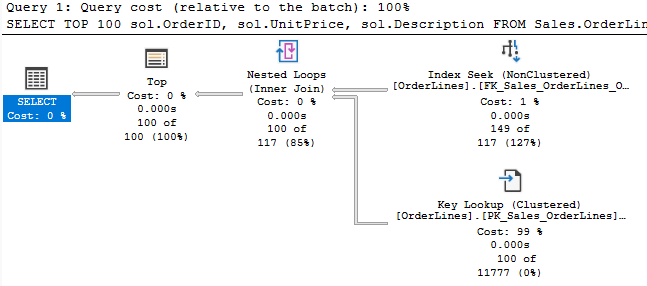
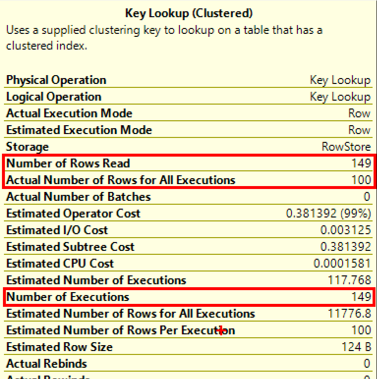
Both Invoices and InvoiceLines have indexes based on InvoiceID, so the data should already be in order. So this should be a good case for a merge (the nested loops below is because of the key lookup on InvoiceLines). But SQL Server’s optimizer still chose nested loops for this query.

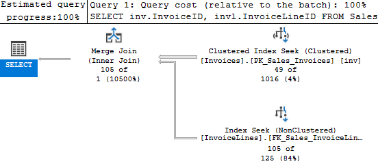
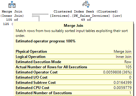
I can hint it to get the behavior I expected, and that plan is below.

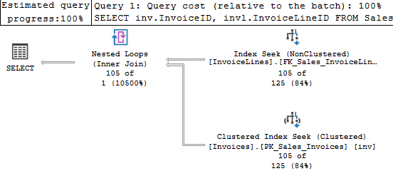
The estimates are way off for the Invoices table, which is odd considering we are seeking on the primary key’s only column; one would expect that estimate to be more accurate. But this estimate causes the cost for the seek against Invoices to be more expensive, so the optimizer chose the other plan. It makes sense.

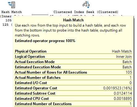
I updated the statistics, and a different plan was chosen. One with a hash match.

???

In that case, the difference in cost was directly the cost of the join operator itself; the cost of the merge join operator was 3x the cost of the hash match operator.

Even if the merge is more efficient, it seems it’s being estimated as being more costly, and specifically for CPU cost. You’re likely to see merge joins much less often than the other two types because of the sort requirement; how it is estimated may also be a factor.

About that sort

The first several times I saw a merge join in an execution plan, the merge was basically the problem with the query. It gave me the impression at the time that merge joins aren’t great in general. But in those cases, the execution plan had a sort after one of the index operations and before the join. Sure, the merge join requires that the two sources be sorted in the same order, but SQL Server could always use a sort operator (expensive as they are) to make that an option.

This seems like an odd choice to make, so let’s consider the following query:

USE WideWorldImporters
GO
SELECT *
FROM Sales.Invoices inv
INNER JOIN Sales.InvoiceLines invl
	ON invl.InvoiceID = inv.InvoiceID
WHERE
	inv.InvoiceDate < DATEADD(month, -12, getutcdate());
GO

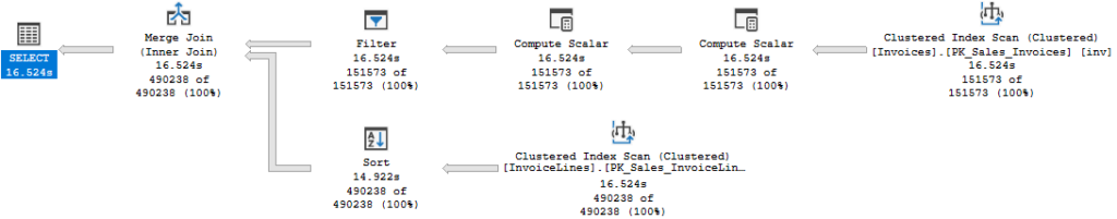
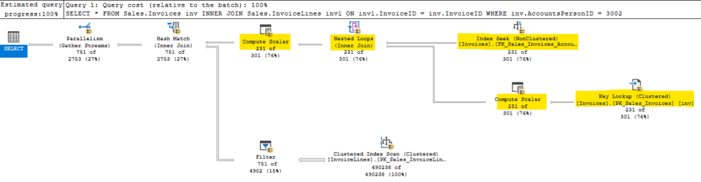
So, this query does a merge join between the two, but there is a sort on the second input. We scan the index, then sort the data to match the other import before we perform the actual join. A sort operator is going to be a large cost to add into our execution plan, so why did the optimizer choose this plan?

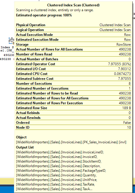
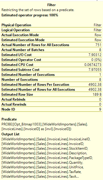
This is a bad query, and the optimizer is trying to create a good plan for it. This may explain many other situations where I have seen a sorted merge. The query is joining the two tables on InvoiceID, and the only filter is on Invoices.InvoiceDate. There is no index on Invoices.InvoiceDate, so it’s a given we’ll scan that table.

If this query used nested loops, we could use the InvoiceID for each record from Invoices to seek a useful index against InvoiceLines, but that would mean we perform 151,578 seeks against that table.

A merge join, even if we have to sort the results from the table, would allow us to perform one index operation instead. But a merge join has to seek independently from the other source, and no other filter is available. So we perform an index scan against the second table as well.

This is probably the best among poor options. To really improve this query, you’d need to add an index or change the WHERE clause.

It took some time for me to realize why I most often saw merge joins in poor execution plans; I wasn’t seeing all the plans using them that perform well. If you are troubleshooting a high CPU situation, when you find the cause you’ll likely be looking at bad plan. We don’t tend to look for the best performing query on the server, do we?

So, if merge join is more efficient than the other two join types in general, we are less likely to be looking at queries where it is being used effectively.

Summary

Hopefully I’ll be getting back to a more regular schedule for the blog. There’s been a number of distractions (an estate sale, mice, etc), but life has been more calm of late (mercifully).

I spoke at the two PASS Summit virtual events over the last two years, and this year I am happy to be presenting in person at PASS Data Community SUMMIT for the first time. So if you are interested in how you can use memory-optimized table variables to improve performance on your system, look out for that session.

When I began working at Microsoft, I was very much a novice at performance troubleshooting. There was a lot to learn, and hash match joins were pointed out to me multiple times as the potential cause for a given issue. So, for a while I had it in my head, “hash match == bad”. But this really isn’t the case.

Hash matches aren’t inefficient; they are the best way to join large result sets together. The caveat is that you have a large result set, and that itself may not be optimal. Should it be returning this many rows? Have you included all the filters you can? Are you returning columns you don’t need?

If SQL Server is using a hash match operator, it could be a sign that the optimizer is estimating a large result set incorrectly. If the estimates are far off from the actual number of rows, you likely need to update statistics.

Let’s look at how the join operates so we can understand how this differs from nested loops

How Hash Match Joins Operate

Build Input

A hash match join between two tables or result sets starts by creating a hash table. The first input is the build input. As the process reads from the build input, it calculates a hash value for each row in the input and stores them in the correct bucket in the hash table.

Creating the hash table is resource intensive. This is efficient in the long run, but is too much overhead when a small number of rows are involved. In that case, we’re better off with another join, likely nested loops.

If the hash table created is larger than the memory allocation allows, it will “spill” the rest of the table into tempdb. This allows the operation to continue, but isn’t great for performance. We’d rather be reading this out of memory than from tempdb.

The building of the hash table is a blocking operator. This means the normal row mode operation we expect isn’t happening here. We won’t read anything from the second input until we have read all matching rows from the build input and created the hash table. In the query above, our build input is the result of all the operators highlighted in yellow.

Probe Input

Once that is complete, we move on to the second input in the probe phase. Here’s the query I used for the plan above:

USE WideWorldImporters
GO

SELECT *
FROM Sales.Invoices inv
INNER JOIN Sales.InvoiceLines invl
	ON invl.InvoiceID = inv.InvoiceID
WHERE
	inv.AccountsPersonID = 3002
GO

The build input performed an index seek and key lookup against Sales.Invoices. That’s what the hash table is built on. You can see from the image above that this plan performs a scan against Sales.InvoiceLines. Not great, but let’s look at the details.

There is no predicate or seek predicate, and we are doing a scan. This seems odd if you understand nested loops, because we are joining based on InvoiceID, and there is an index on InvoiceID for this table. But the hash match join operated differently, and doesn’t iterate the rows based on the provided join criteria. The seek\scan against the second table has to happen independently, then we probe the hash table with the data it returns.

If the read against Sales.InvoiceLines table can’t seek based on the join criteria, then we have no filter. We scan the table, reading 490,238 rows. Also unlike a nested loop join, we perform that operation once.

There is a filter operator before the hash match operator. For each row we read of Sales.InvoiceLines, we create a hash value, and check against the hash table for a match. The filter operator reduces our results from 490,238 rows to 751, but doesn’t change the fact that we had to read 490,238 rows to start with.

In the case of this query, I’d want to see if there’s a filter I can apply to the second table. Even if it doesn’t change our join type away from a hash match, if we performed a seek to get the data initially from the second table, it would make a huge difference.

Remember Blocking Operators?

I mentioned the build input turns that branch of our execution plan into a blocking operator. This is something try to call out the normal flow of row mode execution.

With a nested loops join, we would be getting an individual row from the first source, and doing the matching lookup on the second source, and joining those rows before the join operator asked the first source for another row.

Here, our hash match join has to gather all rows from the first source (which here includes the index seek, key lookup, and nested loops join) before we build our hash table. This could significantly affect a query with a TOP clause.

The TOP clause stops the query requesting new rows from the operators underneath it once it has met it’s requirement. This should result in reading less data, but a blocking operator forces us to read all applicable rows first, before we return anything to upstream operators.

So if your TOP query is trying to read a small number of rows but the plan has a hash match in it, you will be likely reading more data that you would with nested loops.

Summary

Actual numbers comparing join types would depend a ton on the examples. Nested loops are better for smaller result sets, but if you are expecting several thousand (maybe ten or more) rows read from a table, hash match may be more efficient. Hash matches are more efficient in CPU usage and logical reads as the data size increases.

I’ll be speaking at some user groups and other events over the next few months, but more posts are coming.

As always, I’m open to suggestions on topics for a blog, given that I blog mainly on performance topics. You can follow me on twitter (@sqljared) and contact me if you have questions. You can also subscribe on the right side of this page to get notified when I post.

Have a good night.

There are a lot of things to know to understand execution plans and how they operate. One of the essentials is understanding joins, so I wanted to post about each of them in turn.

The three basic types of join operators are hatch match, merge, and nested loops. In this post, I’m going to focus on the last, and I will post on the other two shortly.

How Nested Loops Operate

Nested loops joins are the join operator you are likely to see the most often. It tends to operate best on smaller data sets, especially when the first of the two tables being joined has a small data set.

In row mode, the first table returns rows one at a time to the join operator. The join operator then performs a seek\scan against the second table for each row passed in from the first table. It searches that table based on the data provided by the first table, and the columns defined in our ON or WHERE clauses.

  • You can’t search the second table independently; you have to have the data from the first table. This is very different for a merge join.
  • A merge join will independently seek or scan two tables, then joins those results. It is very efficient if the results are in the same order so they can be compared more easily.
  • A hash join will seek or scan the second table however it can, then probes the hash table with values from the second table based on the ON clause.

So, if the first table returns 1,000 rows, we won’t perform an index seek (or scan) against the second; we will perform 1,000 seeks (or scans) against that index, looking for any rows that relate to the row from the first table.

The query above joins several table, using nested loops between each. we can see that the row counts for the first several tables are all 1. We read one SalesPerson record, the related SalesTerritory, an Employee record, and a Person record. When we join that to the SalesOrderHeader table, we find 234 related rows. That comes from 1 index seek, as internal result set only had 1 row thus far. If we join to LineItem next, we would perform that seek 234 times.

Key Lookups

The optimizer always uses nested loops for key lookups, so you’ll see them frequently for this purpose. I was unsure if this was the only way key lookups are implemented, but this post from Erik Darling confirms it.

In the plan above, we return 149 rows from OrderLines table. We use a nested loops join operator so we can include the UnitPrice and Description in our output, since they aren’t in the nonclustered index.

Which means we execute the key lookup 149 times. The cost for this operator is 99% of the total query, but the optimizer overestimated how many rows we would return.

I frequently look at key lookups as an opportunity for tuning. If you look at the output for that operator, you can see which columns are causing the key lookup. You can either add those columns to the index you expect this query to use (as included columns), or you can ask whether those columns really need to be included in the query. Either approach will remove the key lookup and the nested loop.

LOOP JOIN hints

You can direct SQL Server to use nested loops specifically in your query by writing the query with (INNER\LEFT\RIGHT\FULL) LOOP JOIN. This has two effects:

  • Forces the optimizer to use the specified join type. This will only force the join type for that specific join.
  • Sets the join order. This forces the tables to be joined in the order they are written (subqueries from WHERE EXISTS clauses are excluded from this). So this point may affect how the others joins operate.

I’ve blogged about using hints previously, so I won’t go on for long on this subject. I like the phrase “With great power comes great responsibility” when thinking about using hints to get a specific behavior. It can be an effective way to get consistent behavior, but you can make things worse if you don’t test and follow up to confirm it works as intended.

Summary

I’ll discuss the other two join types in another post. In short, hash matches are more efficient for large data sets, but the presence of a large data set should make us ask other questions. Merge joins are very efficient when dealing with data from two sources that are already in the same order, which is unlikely in general.

Thanks to everyone who voted for my session in GroupBy. I enjoyed speaking at the event, and had some interesting discussion and questions. I expect recordings for the May event will be available on GroupBy’s Youtube page, so keep an eye out for that if you missed the event.

As always, I’m open to suggestions on topics for a blog, given that I blog mainly on performance topics. You can follow me on twitter (@sqljared) and contact me if you have questions. You can also subscribe on the right side of this page to get notified when I post.

Hope you are all enjoying a long weekend.