Estimates and statistics are often discussed in our community, but I doubt the average DBA knows how they flow. So I wanted to write a post with examples showing how SQL Server estimates the rows for a specific operation.
Statistics
The SQL Server optimizer will estimate how many rows it expects to return for a query using statistics. This is part of how it determines the cost of plans and decides which plan to use.
Let’s take a look at the statistics for the Sales.Order table in the WideWorldImporters database. There is an index on the CustomerID column, so we’ll look at the statistics for that object.
DBCC SHOW_STATISTICS('Sales.Orders', FK_Sales_Orders_CustomerID);
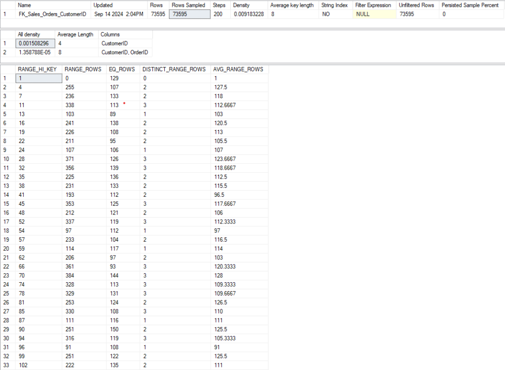
Here’s most of the result from the DBCC command:
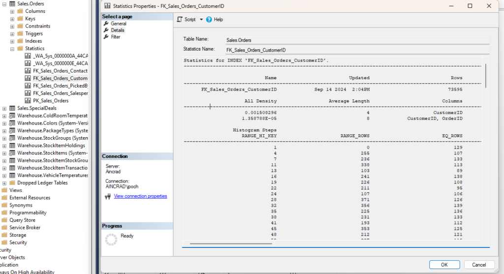
You can also get the same information by double-clicking the statistic in SSMS, and going to Detail on the popup:
Let’s look at the most important elements.
- Updated: Very important. How often you should update statistics depends on several factors, but it’s good to know how old your statistics are when troubleshooting a bad plan. This date is from 2016 if you’ve just restored the WideWorldImporters database, but I just rebuilt that index (which updates the stats with a 100% sampling rate for free).
- Rows and Rows Sampled: How many rows are in the index, and how many were sampled for the statistic object. This is a 100% sampling rate, but when stats are updated automatically this number can easily be less than 1%. The lower the sampling rate, the less accurate the statistics will be. This can lead to bad decisions by the optimizer. I prefer a higher rate, but we have to decide how long we want this to take on a large table.
- Steps: Each step contains information about a range of key values for the index. Each step is defined by the last range value included. The final output shows each step as a row. 200 is the maximum number of steps.
- All Density: This number is the inversion of the number of unique values for this column (1/distinct values). If the key has multiple columns, this will have multiple rows, and you can see how much more selective the index is when the additional columns are included. The value of 0.001508296 corresponds to 663 unique CustomerID values in the index. There are multiple rows in the second result set because this index has multiple columns. The All Density value gives the uniqueness for each combination of columns.
The third result set is a bit more involved, so I wanted to discuss how we can use it.
Histogram
- RANGE_HI_KEY: Indicates the highest value for this range of values, as each row represents a step I referenced earlier. There is a row with a RANGE_HI_KEY of 3, and the next row is 6. This means CustomerID 4 and 5 are in the same step as 6, which is the RANGE_HI_KEY.
- RANGE_ROWS: Gives the number of rows for all values of this step\range, excluding the RANGE_HI_KEY.
- EQ_ROWS: Gives the number of rows equal to the RANGE_HI_KEY.
- DISTINCT_RANGE_ROWS: This gives how many distinct values there are in the RANGE_ROWS, excluding the RANGE_HI_KEY again.
- AVG_RANGE_ROWS: How many values are there for a key value in this range, on average.
Looking at the third row where the RANGE_HI_KEY is 6, the EQ_ROWS are 106. So if we query for CustomerID = 6, this histogram tells us we should return 106 rows.
The DISTINCT_RANGE_ROWS is 2, so there is only one more CustomerID in this range (either 4 or 5). RANGE_ROWS is 214, so the other CustomerID should have 108 rows, but if there are more than 2 distinct values we won’t know any number besides the EQ_ROWS. So if we look up a range value that isn’t the RANGE_HI_KEY, we’ll estimate based on AVG_RANGE_ROWS.
Example #1: RANGE_HI_KEY
To see how these numbers are used, let’s look at a simple query against the Sales.Orders table.
--RANGE_HI_KEY and EQ_ROWS
SELECT
	OrderID
FROM Sales.Orders so
WHERE
	so.CustomerID = 99;
GO
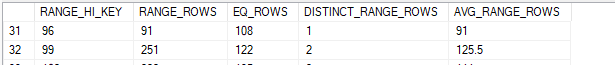
Since 99 is the RANGE_HI_KEY for its step, we just need to check the EQ_ROWS. This query should return 122 rows. Since 99 is the RANGE_HI_KEY for its step, we just need to check the EQ_ROWS. This query should return 122 rows.
So let’s look at the plan to confirm.
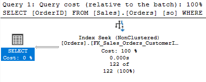
That’s the estimate the plan displays, and it’s accurate because I just updated my stats.
Example #2: AVG_RANGE_ROWS
Slightly different if we search for a value that is not the RANGE_HI_KEY for its step.
--RANGE_HI_KEY and AVG_RANGE_ROWS
SELECT
	OrderID
FROM Sales.Orders so
WHERE
	so.CustomerID = 98;
GO
Each step is defined by its highest value. So if there is a step for 96 and 99, 98 is in the same step as 99. We don’t know the number of rows for any row in the step except for the RANGE_HI_KEY, so the estimate should be the value stored in AVG_RANGE_ROWS, 125.5.
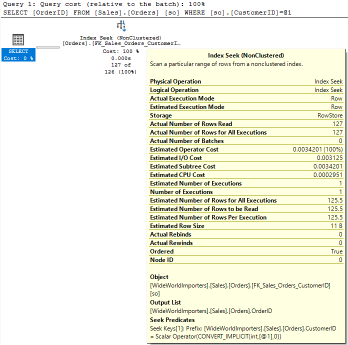
The operator indicates an estimate of 126, but if we hover over it we can see the exact value of 125.5. We returned 127 rows. There are limitations here, but this is a pretty close estimate.
Exampled #3: Variables
We see a different behavior if we use a variable in the query.
--Variable Estimate
DECLARE @CustomerID INT = 99;

SELECT
	OrderID
FROM Sales.Orders so
WHERE
	so.CustomerID = @CustomerID;
GO
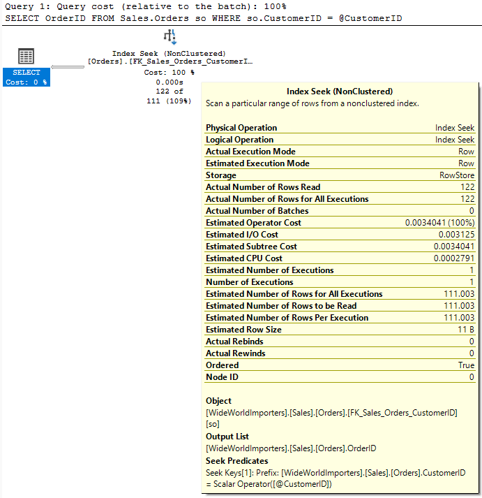
The estimate is off. When we had the value inline, the optimizer “sniffed” that value to see how many rows to expect. It didn’t do the same for the local variable.
Since the optimizer doesn’t know what the value inside that variable is, it can’t use the histogram. It has to make an estimate based on the details at the table level instead of the step level.
I mentioned the All Density value earlier. It’s a measure of how unique a given column is. If you multiply that value by the number of rows in the table, you should get an average number of rows that would be returned for a given CustomerID.
--Calculated Estimate
DECLARE
	@density numeric(12,12) = 0.009183228,
	@all_density numeric (12,12) = 0.001508296,
	@rows int = 73595.

SELECT
	1.0/@all_density AS Distinct_CustomerID,
	@all_density * @rows AS Estimated_Rows;
GO
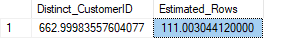
This matches the value of 111.003 from the execution plan. So this is a somewhat blind estimate for any CustomerID when the optimizer doesn’t know the value before compiling.
Sidenote on Example #3:
This didn’t calculate correctly for me at first. It caused much consternation as I did more reading to try to understand why the numbers didn’t match. I likely would have posted this blog some time ago without this issue.
Then I realized WideWorldImporters was created for SQL Server 2016. These statistics were created in SQL Server 2016, and were restored with the rest of the database on my instance of SQL Server 2022.
Maybe I should rebuild the index? Then I did. And now it works perfectly.
Something to keep in mind for your endeavors.
Exampled #4: RECOMPILE
If we add OPTION(RECOMPILE) to our query, the optimizer will sniff the local variable and
--Recompile to Sniff Local Variable
DECLARE @CustomerID INT = 99;

SELECT
	OrderID
FROM Sales.Orders so
WHERE
	so.CustomerID = @CustomerID
OPTION(RECOMPILE);
GO
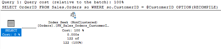
And now our estimate is accurate again. It’s good to understand this point because you may see a large difference if you use OPTION(RECOMPILE) with a query that depends on a local variable.
Range Estimates
With range seeks (inequality comparisons), things are a bit different. We’re not looking for a specific value, and we’ll use our statistics differently. And there is one issue I’d like to point out. Consider this query:
SELECT so.OrderID
FROM Sales.Orders so
WHERE
	so.CustomerID >= 1001;
GO
When I execute this, the estimate is very accurate.
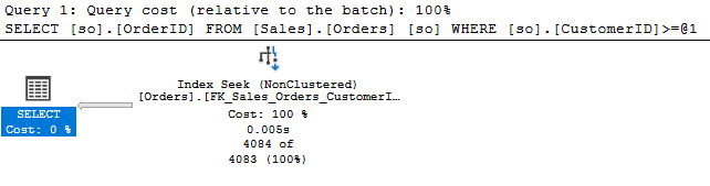
We’re only off by 1 row, and I will happily accept. But how did the optimizer arrive here? Let’s look at the last group of steps in this statistic.
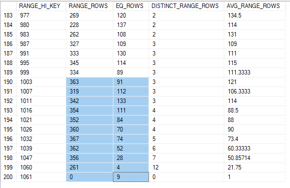
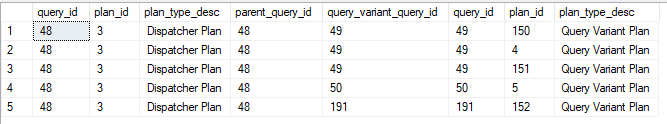
The RANGE_ROWS is useful to use here for this range seek. It will tell the optimizer how many rows to expect from each step, but it excludes the EQ_ROWS, which is the number of rows for the RANGE_HI_KEY itself. So, to estimate this we will need to include the EQ_ROWS and RANGE_ROWS for each of these steps. If you add the highlighted numbers, you’ll end up with 4204.
Of course, the query would exclude CustomerID 1000, which should be in the step for CustomerID 1003. We don’t the exact value for this CustomerID; it’s one of our range values. So our best estimate is the AVG_RANGE_ROWS for that step, 121. If we subtract the 121 rows we estimate for CustomerID 1000, we have a final estimate of 4083.
Inequalities and Variables
But what if you used a variable with that same query?
DECLARE @CustomerID INT = 1001;

SELECT so.OrderID
FROM Sales.Orders so
WHERE
	so.CustomerID >= @CustomerID;
GO
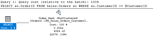
The estimate is off by 82%. What just happened?
The optimizer can’t probe the variable, so it has nothing to base its estimate on. This estimate of 22078 is a default the optimizer uses guessing our query will return 30% of the rows in the table. This is present in the legacy cardinality estimator and the current CE for SQL Server 2022.
The first time I heard of this estimate was at a talk at PASS Summit. There are some references to it on other blogs, but there aren’t many of them.
These two blogs by Erik Darling and Andrew Pruski refer to the 30% estimate, and if you are reading this blog you might find them enlightening.
This blog by @sqlscotsman has more details about estimates and guesses involving other operators including LIKEs and BETWEENs.
In a more complex query where the range seek isn’t the only option to filter on, SQL Server can use other fields to make a more accurate estimate.
In Summary
Why does accuracy matter? When estimates are inaccurate, SQL Server will compare plans with incorrect costs. We’re more likely to end up with bad plans that over\under allocate resources or use the wrong join type or join order for a query.
The wrong plan can multiply the runtime of a query many times and massive increase blocking issues.
Knowing how our statistics function can help us write better procedures that are less likely to leave the optimizer in the dark.
My social media links are above. Please contact me if you have questions, and I’m happy to consult with you if you have a more complex performance issue. Also, let me know if you have any suggestions for a topic for a new blog post.