I wrote about Parameter Sensitive Plan Optimization in my last blog. In this post, I want to talk about a specific problem you may see in Query Store, depending on how to get information from it.
A Query Store Example
I use Query Store frequently, and I tend to be working on a specific stored procedure at a time. Either I’m evaluating a procedure to see how we can improve its performance, or I’m testing\validating the improvements to that procedure. Here’s an example Query Store script I might use.
SELECT
	qsq.query_id,
	qsp.plan_id,
	CAST(qsp.query_plan as XML) AS query_plan,
	qt.query_sql_text,
	rsi.end_time,
	(rs.avg_duration * rs.count_executions) as total_duration,
	rs.avg_duration,
	rs.count_executions,
	rs.avg_cpu_time,
	rs.avg_logical_io_reads,
	rs.avg_rowcount
FROM sys.query_store_query qsq
INNER JOIN sys.query_store_plan qsp
	ON qsp.query_id = qsq.query_id
INNER JOIN sys.query_store_query_text qt
	ON qt.query_text_id = qsq.query_text_id
INNER JOIN sys.query_store_runtime_stats rs
	ON rs.plan_id = qsp.plan_id
INNER JOIN sys.query_store_runtime_stats_interval rsi
	ON rsi.runtime_stats_interval_id = rs.runtime_stats_interval_id
WHERE
	qsq.object_id = OBJECT_ID('dbo.User_GetByReputation')
	AND rsi.end_time > DATEADD(DAY,-2, GETUTCDATE())
This query gets the execution stats from the procedure I used in my last blog post against the StackOverflow2013 database. Any executions in the last two days will be included in the results.
Or it should. When I run this I get “(0 rows affected)”.
But I just ran this procedure, so what’s the issue?
sys.query_store_query_variant
This is an example of a query that needs to be updated for SQL Server 2022 with Parameter Sensitive Plan Optimization in place, and the reason has to do with changes made to allow variant queries.
There is a new table in Query Store that is essential to the PSPO feature: sys.query_store_query_variant.
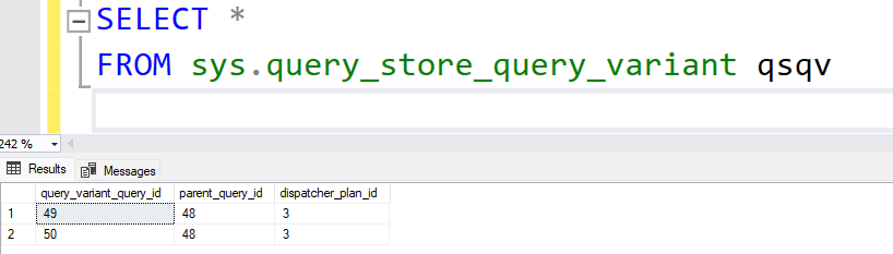
The table is something of a stub, with only three columns. This establishes the relationship between the parent query, variant queries, and the dispatcher plan.
You can see in this case there are two variants for the same parent_query_id. So, for a given query you could LEFT JOIN to sys.query_store_query_variant to find any variant queries it may have, then join back to sys.query_store_query to get the rest of the details for that variant query.
Parent Queries Don’t Execute
But why did my query have no results?
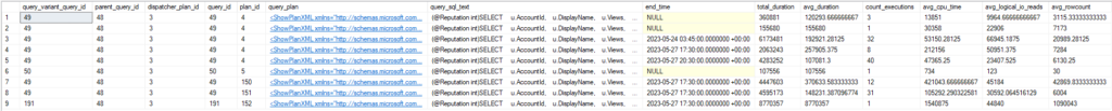
The first issue is that the parent queries and the plan associated with them don’t execute. Joining the tables that give the query, plan, and text is fine, but when we INNER JOIN sys.query_store_runtime_stats and sys.query_store_runtime_stats_interval we lose our results.
Running the same query with LEFT JOINs shows the execution stats are all NULL.

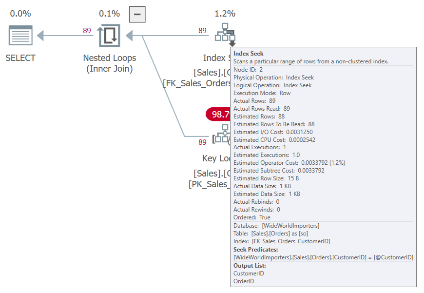
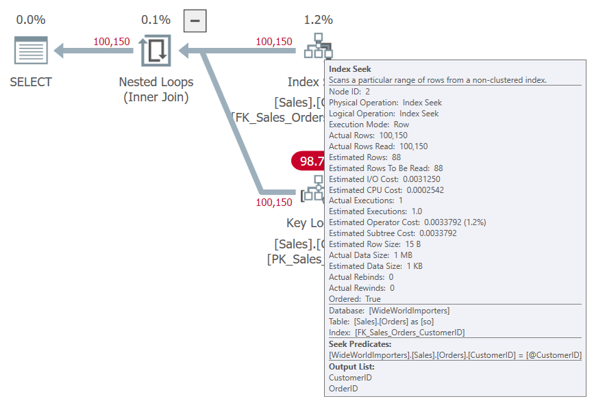
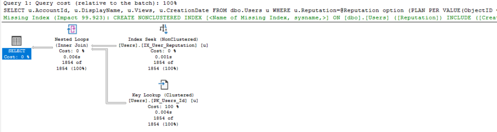
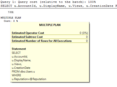
While we are here, if I click on the link for the plan I will see the dispatcher plan. This isn’t a full execution plan, but there is some information about the use of PSPO (the boundaries and details of the statistic used) in the XML.
<ShowPlanXML xmlns="http://schemas.microsoft.com/sqlserver/2004/07/showplan" Version="1.564" Build="16.0.1050.5">
<BatchSequence>
<Batch>
<Statements>
<StmtSimple StatementText="SELECT 
 u.AccountId,
 u.DisplayName,
 u.Views,
 u.CreationDate
 FROM dbo.Users u
 WHERE 
 u.Reputation=@Reputation" StatementId="1" StatementCompId="3" StatementType="MULTIPLE PLAN" RetrievedFromCache="false" QueryHash="0x08FD84B17223204C" QueryPlanHash="0x86241E8431E63362">
<Dispatcher>
<ParameterSensitivePredicate LowBoundary="100" HighBoundary="1e+06">
<StatisticsInfo LastUpdate="2023-05-19T14:04:14.91" ModificationCount="0" SamplingPercent="100" Statistics="[IX_User_Reputation]" Table="[Users]" Schema="[dbo]" Database="[StackOverflow2013]" />
<Predicate>
<ScalarOperator ScalarString="[StackOverflow2013].[dbo].[Users].[Reputation] as [u].[Reputation]=[@Reputation]">
<Compare CompareOp="EQ">
<ScalarOperator>
<Identifier>
<ColumnReference Database="[StackOverflow2013]" Schema="[dbo]" Table="[Users]" Alias="[u]" Column="Reputation" />
</Identifier>
</ScalarOperator>
<ScalarOperator>
<Identifier>
<ColumnReference Column="@Reputation" />
</Identifier>
</ScalarOperator>
</Compare>
</ScalarOperator>
</Predicate>
</ParameterSensitivePredicate>
</Dispatcher>
</StmtSimple>
</Statements>
</Batch>
</BatchSequence>
</ShowPlanXML>
But if we didn’t execute the dispatcher plan for the parent query, we should have executed the plan for the variant query. Why didn’t we see that in our results?
Variant Queries’ Object_ID = 0 (Adhoc)
The second issue is that variant queries have an object_id of 0 in sys.query_store_query; the same as an ad-hoc query.
I was filtering on the object_id of my procedure to only get results for that procedure, but that doesn’t include our variant queries.
But I can query from the sys.query_store_query_variant table to sys.query_store_query based on the query_variant_query_id to get the details for my variant query, then join to other tables to get the stats I was looking for.
SELECT
	var.*,
	qsq.query_id,
	qsp.plan_id,
	CAST(qsp.query_plan as XML) AS query_plan,
	qt.query_sql_text,
	rsi.end_time,
	(rs.avg_duration * rs.count_executions) AS total_duration,
	rs.avg_duration,
	rs.count_executions,
	rs.avg_cpu_time,
	rs.avg_logical_io_reads,
	rs.avg_rowcount
FROM sys.query_store_query_variant var
INNER JOIN sys.query_store_query qsq
	ON qsq.query_id = var.query_variant_query_id
INNER JOIN sys.query_store_plan qsp
	ON qsp.query_id = qsq.query_id
LEFT JOIN sys.query_store_query_text qt
	ON qt.query_text_id = qsq.query_text_id
LEFT JOIN sys.query_store_runtime_stats rs
	ON rs.plan_id = qsp.plan_id
LEFT JOIN sys.query_store_runtime_stats_interval rsi
	ON rsi.runtime_stats_interval_id = rs.runtime_stats_interval_id
	AND rsi.end_time > DATEADD(DAY,-2, GETUTCDATE());
Getting the runtime statistics isn’t the hard part, it’s just identifying which queries we care about.
Silent Failure
If you use Query Store regularly, and especially if you have any tools or automation built on that information, you’ll need to account for the two points above. Because your existing scripts won’t fail, they will give you incomplete results. This is a case where an actual error would be more helpful; you’d know something had broken.
So, how do we get all the execution details for our procedure? First, let’s see the parent query and its children (updated per the addendum).
SELECT
	qsq.query_id,
	qsp.plan_id,
	qsp.plan_type_desc,
	vr.parent_query_id,
	vr.query_variant_query_id,
	qv.query_id,
	qvp.plan_id,
	qvp.plan_type_desc
FROM sys.query_store_query qsq
INNER JOIN sys.query_store_plan qsp
	ON qsp.query_id = qsq.query_id
LEFT JOIN sys.query_store_query_variant vr
	ON vr.parent_query_id = qsq.query_id
    AND vr.dispatcher_plan_id = qsp.plan_id
LEFT JOIN sys.query_store_query qv
	ON qv.query_id = vr.query_variant_query_id
LEFT JOIN sys.query_store_plan qvp
	ON qvp.query_id = qv.query_id
WHERE
	qsq.object_id = OBJECT_ID('dbo.User_GetByReputation');
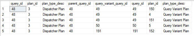
Also, note that sys.query_store_plan has two new columns that are relevant to us; plan_type_desc and plan_type. Query_id 48 is the parent query related to the “Dispatcher Plan”; the variant plan is marked as “Query Variant Plan”. A normal plan would be a “Compiled Plan”.
A Suggested Solution
We could return both, but we don’t really need to. The parent query has no related performance statistics, but we need the parent query to find all the variant queries that allow us to get the execution statistics.
There is one more issue to consider; sys.query_store_query_variant does not exist in a SQL Server instance below 2022. So if we want a procedure that can run on our un-upgraded instances, we’ll need two paths.
Oh, we also want to make sure we don’t miss plans for any queries not using PSPO.
Here’s a simple procedure that does that (which has been updated per the addendum).
USE StackOverflow2013
GO
CREATE OR ALTER PROCEDURE dbo.QS_GetProcedurePerfDetails
  @Schema_Object NVARCHAR(100),
  @StartDate DATETIME2
AS
	DECLARE
		@c_level INT,
		@obj_id INT;

	CREATE TABLE #QueryList (
		query_id INT,
		plan_id INT,
		query_plan NVARCHAR(MAX),
		query_text_id INT,
		plan_type_desc NVARCHAR(120) NULL
	);

	SELECT
		@c_level = db.compatibility_level
	FROM sys.databases db
	WHERE
		db.database_id = DB_ID();

	SET @obj_id = OBJECT_ID(@Schema_Object);

	-- Based on the compatability level, get IDs for relevant queries and plans
	IF (@c_level < 160)
	BEGIN
		INSERT #QueryList
		SELECT
			qsq.query_id,
			qsp.plan_id,
			qsp.query_plan,
			qsq.query_text_id,
			NULL AS plan_type_desc
		FROM sys.query_store_query qsq
		INNER JOIN sys.query_store_plan qsp
			ON qsp.query_id = qsq.query_id
		WHERE
			qsq.object_id = @obj_id;
	END
	ELSE
	BEGIN
		INSERT #QueryList
		SELECT
			ISNULL(qv.query_id,qsq.query_id) AS query_id,
			ISNULL(qvp.plan_id,qsp.plan_id) AS plan_id,
			ISNULL(qvp.query_plan,qsp.query_plan) AS query_plan,
			ISNULL(qv.query_text_id,qsq.query_text_id) AS query_text_id,
			ISNULL(qvp.plan_type_desc,qsp.plan_type_desc) AS plan_type_desc
		FROM sys.query_store_query qsq
		INNER JOIN sys.query_store_plan qsp
			ON qsp.query_id = qsq.query_id
		LEFT JOIN sys.query_store_query_variant vr
			ON vr.parent_query_id = qsq.query_id
            AND vr.dispatcher_plan_id = qsp.plan_id
		LEFT JOIN sys.query_store_query qv
			ON qv.query_id = vr.query_variant_query_id
		LEFT JOIN sys.query_store_plan qvp
			ON qvp.query_id = qv.query_id
		WHERE
			qsq.object_id = @obj_id;
	END;

	SELECT
		ql.query_id,
		ql.plan_id,
		ql.plan_type_desc,
		CAST(ql.query_plan as XML),
		qt.query_sql_text,
		rsi.end_time,
		(rs.avg_duration * rs.count_executions) as total_duration,
		rs.avg_duration,
		rs.count_executions,
		rs.avg_cpu_time,
		rs.avg_logical_io_reads,
		rs.avg_rowcount
	FROM #QueryList ql
	INNER JOIN sys.query_store_query_text qt
		ON qt.query_text_id = ql.query_text_id
	LEFT JOIN sys.query_store_runtime_stats rs
		ON rs.plan_id = ql.plan_id
	LEFT JOIN sys.query_store_runtime_stats_interval rsi
		ON rsi.runtime_stats_interval_id = rs.runtime_stats_interval_id
	WHERE
		rsi.end_time > @StartDate
	ORDER BY
		qt.query_sql_text,
		rsi.end_time;
GO

EXEC dbo.QS_GetProcedurePerfDetails
  @Schema_Object = 'dbo.User_GetByReputation',
  @StartDate = '2023-05-24';
GO
I’m checking to see if the compatibility level is at least 160 as a way to see if we are on SQL Server 2022 or not. Of course, we could be using SQL Server 2022 with a lower compatibility level, but the sys.query_store_query_variant table would be empty in that case.
The key is to have an initial step to get the queries and plans we want. This has a LEFT JOIN to sys.query_store_query_variant in case there are variant queries to consider. We join to get the other details for the variant (the query_text_id, plan_id, and the plan itself) if they exist.
I’m throwing those initial results in a temp table to use in the final query. I’ve also found in my testing that splitting this operation in two helps to prevent the plan from getting too large and sluggish.
The temp table is populated with the details of the variant query and its “Query Variant Plan”, if present, but if they are NULL we use the details of what must be a normal query with a “Compiled Plan”.
From here, you can also get more complex and include options to aggregate the Query Store details or include more columns, but this should solidify how to incorporate sys.query_store_query_variant into your scripts.
In Summary
This is something I’ve been working on for a while. It became obvious to me months ago that we needed to include this logic at work so that our own Query Store aggregation wouldn’t suddenly miss a lot of executions.
Hopefully, this post will help some readers to avoid this pitfall.
You can follow me on Twitter (@sqljared) and contact me if you have questions. My other social media links are at the top of the page. Also, let me know if you have any suggestions for a topic for a new blog post.
Addendum
As I pointed out in my next post, the join I originally made to sys.query_store_query_variant was incorrect. If you only join based on the query_id, the result set gets multiplied. Each variant query is shown as related to all plans for the parent query, even “compiled plan” type plans which do not use PSPO at all.
I’ve updated the scripts above in two places, but wanted to call that out.